Statistics and machine learning
Handling Imbalanced Data in Credit Risk Models
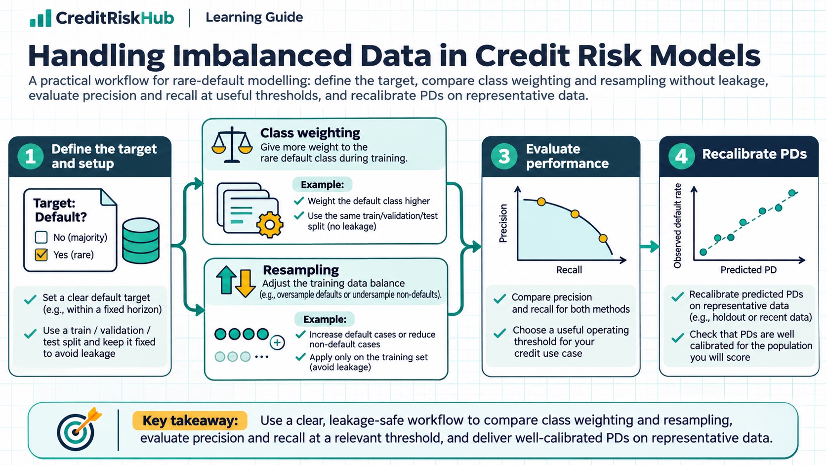
A practical workflow for rare-default modelling: define the target, compare class weighting and resampling without leakage, evaluate precision and recall at useful thresholds, and recalibrate PDs on representative data.
Updated 2026-10-25
Purpose
A practical workflow for rare-default modelling: define the target, compare class weighting and resampling without leakage, evaluate precision and recall at useful thresholds, and recalibrate PDs on representative data.
Key terms
Hover over or focus a term for a quick definition, or open its glossary entry.
• Recall (sensitivity) = true positives / (true positives + missed defaults). It measures the share of defaults found.
• Precision = true positives / (true positives + false alarms). It measures how many flagged borrowers actually defaulted.
• Specificity = true negatives / (true negatives + false alarms). It measures the share of non-defaults not flagged.
• Balanced accuracy = (recall + specificity) / 2. It gives each class equal weight, but it does not measure PD calibration or business value.
Precision = 12 / (12 + 98) = 10.9%.
Recall = 12 / (12 + 8) = 60.0%.
Specificity = 882 / (882 + 98) = 90.0%.
Accuracy = (12 + 882) / 1,000 = 89.4%.
PURPOSE
Defaults are rare in many lending portfolios. That can make a classifier look accurate while missing most defaults, and it can make probability estimates difficult to validate. This guide gives a step-by-step way to diagnose class imbalance, test possible treatments, and keep probability of default (PD) estimates meaningful. All examples use synthetic data.
The goal is not to make the classes look equal. The goal is to produce useful, well-evaluated estimates for the real portfolio and intended decision. Imbalance treatment is a modelling choice that must be justified with out-of-time evidence.
1. DEFINE THE CREDIT-RISK TARGET FIRST
Choose the unit (obligor, facility, or application), observation date, default definition, performance window, eligibility rules, and label-maturity date. For an application PD model, specify what counts as default within the stated horizon, such as default within 12 months of origination. Keep these definitions consistent with the model’s intended use.
Build features using only information available at the observation date. Keep future outcomes, post-default collections, later status updates, and downstream decisions out of the predictors. If one borrower has multiple facilities or applications, decide how they are grouped so records from the same borrower do not leak across training and validation partitions. Split chronologically when the production use predicts future applicants, and reserve a final out-of-time test set.
Do not count an account with an incomplete performance window as a non-default. Mark it immature or handle censoring with a method suited to the target. Report the number of eligible records, defaults, and mature outcomes in every partition.
2. ESTABLISH THE NATURAL-PREVALENCE BASELINE
Calculate the default rate in each chronological partition before changing anything. Fit a simple baseline model using the natural training population, then evaluate it on untouched validation data with the natural class mix. Check data quality, duplicates, label errors, time drift, and selection effects before attributing poor results to imbalance.
Accuracy alone is misleading when defaults are uncommon. If 2% of 1,000 borrowers default, a rule that predicts “no default” for everyone is 98% accurate and has zero default recall. Always compare a proposed model with this simple baseline.
3. CHOOSE METRICS THAT MATCH THE DECISION
Start with the event prevalence and the confusion matrix at each candidate decision threshold. The positive class here is default.
• The precision-recall curve shows precision and recall across thresholds. Average precision summarizes points on this curve; report the definition used because it is not always identical to trapezoidal area. Include the default-rate baseline so readers can interpret the result.
• ROC-AUC can describe ranking across thresholds, but supplement it with precision-recall results when defaults are rare. Neither AUC nor average precision tells you whether predicted PDs are calibrated.
Pick operating points using real constraints: review capacity, customer impact, the cost of false alarms, and losses from missed defaults. Report “recall at a fixed review rate” or “precision at a target recall” where appropriate. The threshold is an operational decision; it is not automatically 50% and it should not be chosen on the final test set.
4. COMPARE TREATMENTS INSIDE THE TRAINING PROCESS
Use a controlled comparison with the same time split, features, model family where possible, and untouched natural-prevalence validation and test cohorts. Try simple choices before complex ones.
A. Keep all records and change the threshold. If ranking is adequate, changing the cutoff may meet a review-capacity target without modifying training data. Compare the workload and the true-positive and false-positive counts at each cutoff.
B. Apply class weights or cost-sensitive loss. Class weights give errors in the minority class more influence during model fitting. This is simple to implement in many algorithms and keeps the original rows. Try several justified weights and compare the trade-off; extreme weights can cause too many false alarms or unstable scores. Record the objective and weighting scheme.
C. Try random undersampling or oversampling. Undersampling discards some majority-class training observations and may lose useful variation. Oversampling repeats minority records and can overfit individual defaults. Test these methods only within each training fold, not before splitting the data.
D. Treat synthetic oversampling cautiously. SMOTE-style methods interpolate minority observations. In credit data, interpolation can create impossible combinations, violate business constraints, or blur meaningful categorical and temporal structure. If a suitable mixed-data method is considered, validate generated records, document constraints, and compare it against simpler methods. Synthetic observations are not new observed defaults.
E. Consider balanced ensembles only when they improve the intended use on untouched data. More complexity brings additional implementation, explanation, and monitoring work. A higher ranking score alone is not enough to justify it.
Never resample the full dataset before creating train and test partitions. That can leak information and produces an evaluation sample whose class mix no longer resembles the production population. Put any sampler inside the cross-validation training pipeline so it is fitted only on each training fold.
5. REASSESS PROBABILITY CALIBRATION
A class-weighted or resampled model may rank borrowers usefully while its raw predicted probabilities no longer represent the natural portfolio’s event rate. Do not present a classifier score or threshold flag as a calibrated PD without checking it.
After selecting a model, fit or assess calibration on a separate, representative cohort with the natural prevalence and fully matured labels. Depending on sample size and stability, compare a sigmoid (Platt-style) calibrator and isotonic calibration. The calibration data must be separate from the data used to fit the base model; time ordering should reflect production use. Isotonic calibration can overfit when calibration outcomes are scarce.
Inspect a reliability diagram by risk band, observed-to-expected defaults, Brier score, and log loss. Brier and log-loss scores combine multiple properties of probabilistic predictions, so do not interpret either as a calibration-only test. For rare defaults, show counts and uncertainty in each band; an attractive portfolio-wide average can hide underprediction in one segment and overprediction in another.
A prior-probability or odds correction is defensible only under a prior-shift assumption: the class-conditional feature distributions stay stable and only event prevalence changes. That assumption can fail when underwriting, customer mix, macroeconomic conditions, or data capture changes. Validate any correction on representative outcomes instead of treating it as a universal fix.
6. WORKED SYNTHETIC EXAMPLE
Suppose an untouched out-of-time cohort has 1,000 mature borrowers and 20 defaults, so natural default prevalence is 2%. At one selected threshold, the model flags 110 borrowers: 12 are defaults and 98 are non-defaults. It misses 8 of the 20 defaults and correctly leaves 882 non-defaults unflagged.
The all-non-default baseline has higher accuracy (98%) but zero recall. That does not prove this model is better: it finds more defaults but also creates 98 false alarms. Whether the trade-off is useful depends on policy, review capacity, costs, customer impact, and the quality of the probability estimates. Compare other thresholds and report how many accounts each one sends to review.
7. COPYABLE PYTHON EXAMPLE — STANDARD LIBRARY ONLY
This deterministic snippet uses the same synthetic confusion matrix. It has no external dependencies, file access, network access, or customer data. Copy the lines into Python 3.
actual = [1] * 20 + [0] * 980
predicted_default = [1] * 12 + [0] * 8 + [1] * 98 + [0] * 882
tp = sum(y == 1 and p == 1 for y, p in zip(actual, predicted_default))
fn = sum(y == 1 and p == 0 for y, p in zip(actual, predicted_default))
fp = sum(y == 0 and p == 1 for y, p in zip(actual, predicted_default))
tn = sum(y == 0 and p == 0 for y, p in zip(actual, predicted_default))
precision = tp / (tp + fp) if tp + fp else 0
recall = tp / (tp + fn) if tp + fn else 0
specificity = tn / (tn + fp) if tn + fp else 0
accuracy = (tp + tn) / len(actual)
print(f'Defaults={sum(actual)} of {len(actual)}; prevalence={sum(actual) / len(actual):.1%}')
print(f'TP={tp}, FN={fn}, FP={fp}, TN={tn}')
print(f'Precision={precision:.1%}; recall={recall:.1%}; specificity={specificity:.1%}; accuracy={accuracy:.1%}')
Expected output: Defaults=20 of 1000; prevalence=2.0%; TP=12, FN=8, FP=98, TN=882; precision=10.9%; recall=60.0%; specificity=90.0%; accuracy=89.4%.
This example calculates one threshold’s hard classifications; it does not calculate a ranking metric or calibrated PD. For threshold analysis, retain model scores and compute the confusion matrix over a grid of cutoffs using the same validation cohort.
8. MONITOR AFTER DEPLOYMENT
Monitor on a scheduled cadence and after material data, policy, model, or portfolio changes. Use stable definitions and compare with a documented baseline.
• Population and label: application volume, default prevalence by vintage and segment, mature-label coverage, missing outcomes, and time since origination.
• Data and pipeline: feature missingness, range and category changes, join rates, duplicate rates, point-in-time availability, scoring failures, and sampler or model version.
• Ranking and operating point: average precision with the prevalence baseline, ROC-AUC as a secondary ranking view, recall, precision, specificity, flagged share, and counts at approved thresholds. Report outcome counts and intervals because rare events make small segments noisy.
• Calibration: observed versus predicted defaults overall and by suitable bands or segments, reliability plots, Brier or log loss, and changes in the calibration mapping. Reassess only on matured, representative outcomes.
• Portfolio and process: approval/decline rates, manual review capacity, overrides, policy changes, collections practice, and evidence of selective outcome observation.
Set investigation triggers based on portfolio size, purpose, uncertainty, and materiality. There is no single threshold that is right for every credit portfolio. A drift or performance alert starts an investigation; it does not automatically require recalibration or model replacement. For low-default portfolios, backtests have limited evidence, so combine them with benchmarking, migration analysis, expert review, and other suitable validation evidence.
9. KEEP THE MEASURE’S PURPOSE CLEAR
A model used for origination screening, an internal risk appetite metric, a Basel regulatory capital estimate, and an IFRS 9 accounting input can have different populations, horizons, definitions, and governance. Changing the training class mix does not change the real portfolio’s default prevalence or an accounting ECL calculation. If a model feeds IFRS 9, validate its probability and cash-shortfall components under the accounting measurement purpose, including appropriate forward-looking information and scenario weighting. Do not substitute a regulatory capital measure or a resampled training rate for an accounting estimate.
PRACTICAL CHECKLIST
1. Define the obligor or facility unit, default event, horizon, eligible population, and maturity rule
2. Use point-in-time features and time-based, borrower-aware partitions
3. Record natural default prevalence in training, validation, and test data
4. Establish an all-majority baseline and report confusion counts
5. Compare threshold choices, class weighting, sampling, and ensembles under the same validation design
6. Keep resampling inside training folds; preserve natural prevalence in validation and test cohorts
7. Choose operating metrics from actual costs, capacity, and customer impact; don’t rely on accuracy alone
8. Recheck calibration on separate, representative, matured outcomes before interpreting scores as PDs
9. Monitor prevalence, label maturity, ranking, threshold performance, calibration, data quality, and process changes
10. State assumptions, uncertainty, limitations, and whether the measure is accounting, regulatory, or internal
REFERENCES
Basel Committee on Banking Supervision, Credit risk – internal ratings-based approach, especially 30.56–30.73 on low-default portfolios and validation: https://www.bis.org/committees/bcbs/basel-consolidated-guidelines/module/cri/30
scikit-learn, Precision-Recall: https://scikit-learn.org/stable/auto_examples/model_selection/plot_precision_recall.html
scikit-learn, Classification metrics: https://scikit-learn.org/stable/modules/model_evaluation.html
scikit-learn, Class weights for imbalanced datasets: https://scikit-learn.org/stable/modules/generated/sklearn.utils.class_weight.compute_sample_weight.html
scikit-learn, Probability calibration: https://scikit-learn.org/stable/modules/calibration.html
imbalanced-learn, Common pitfalls and recommended practices (resampling leakage): https://imbalanced-learn.org/stable/common_pitfalls.html
IFRS Foundation, IFRS 9 Financial Instruments: https://www.ifrs.org/issued-standards/list-of-standards/ifrs-9-financial-instruments/
Educational material only. All values and records are synthetic. The example is not a credit decision rule. Validate target definitions, methodology, model governance, customer impacts, and accounting or regulatory requirements for the specific use case.
Try a reproducible Python example
These examples use synthetic inputs and run locally in a browser worker. Edit the code, run it, and compare its output with the published example.
Runnable Python · local in your browser
Calculate WOE and IV from grouped counts
Use synthetic good and bad counts for three ordered scorecard bins. The 0.5 adjustment avoids a zero distribution in this small example.
Output
Run the code to see the output.
Runtime loads only after you press Run. Code runs in a separate browser worker with a 10-second limit and a 20,000-character output cap. Use synthetic examples only; browser execution is not a secure environment for secrets or sensitive records.
Runnable Python · local in your browser
Convert a logistic model logit to PD
Apply the logistic function to an illustrative intercept plus two feature contributions.
Output
Run the code to see the output.
Runtime loads only after you press Run. Code runs in a separate browser worker with a 10-second limit and a 20,000-character output cap. Use synthetic examples only; browser execution is not a secure environment for secrets or sensitive records.
References
- Basel Committee; scikit-learn; imbalanced-learn; IFRS Foundation — Basel Committee; scikit-learn; imbalanced-learn; IFRS Foundation
Educational material only. Methods and examples are simplified; state and validate the assumptions required for your use case.