Statistics and machine learning
Calibrating probability models
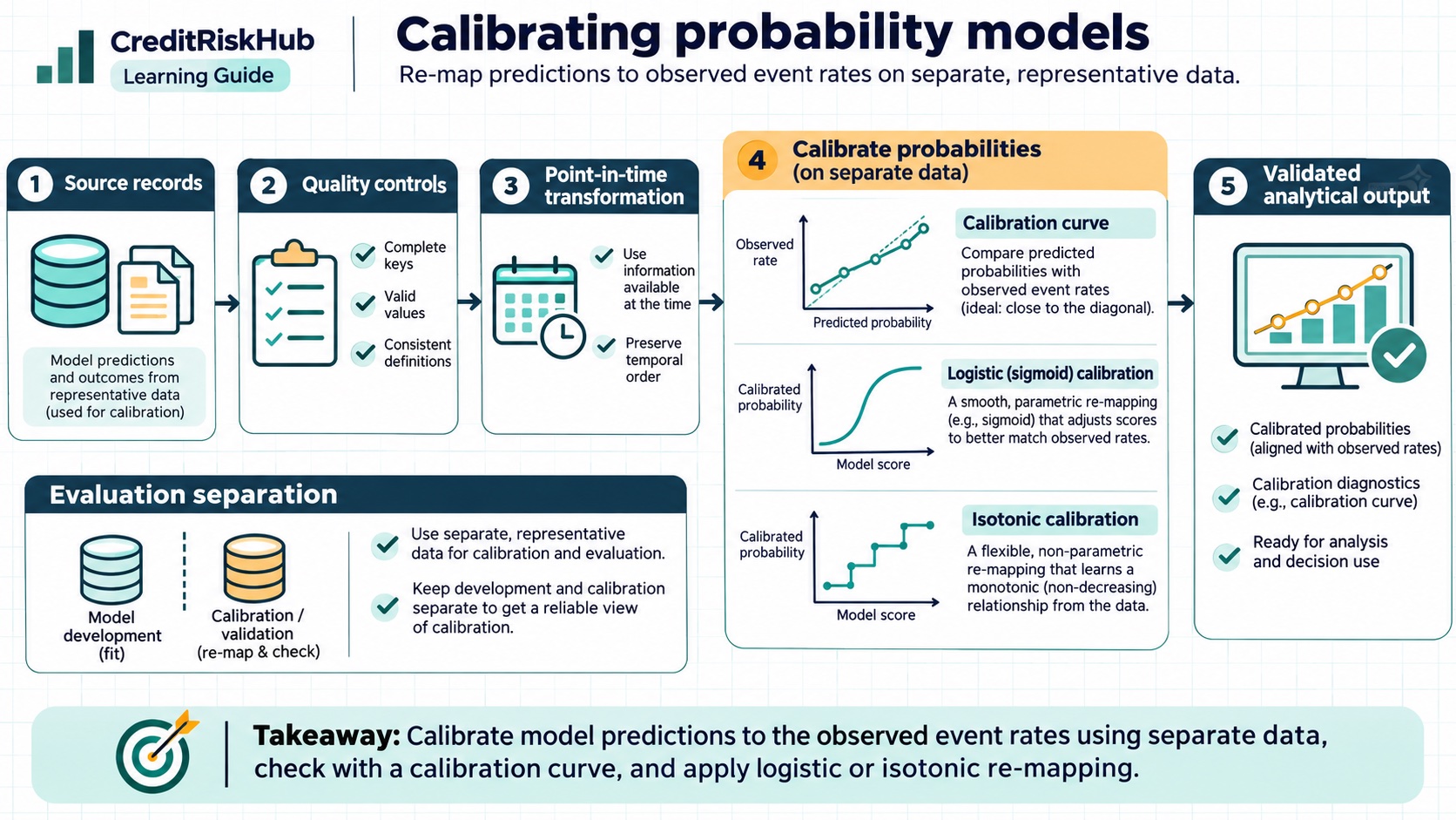
Re-map predictions to observed event rates on separate, representative data.
Purpose
Explain calibration curves, logistic/sigmoid calibration, isotonic calibration, and evaluation separation.
Key terms
Hover over or focus a term for a quick definition, or open its glossary entry.
Key definitions
- A calibrated probability aligns predicted probabilities with observed event frequencies over a defined population and horizon.
- Calibration is distinct from ranking or discrimination.
For a calibrated group, mean predicted PD should be compared with observed default frequency over the matched horizon.Worked example
Among 500 accounts assigned an average PD near 2%, about 10 defaults are expected on average under a comparable target population, not as a guaranteed count.
Detailed explanation
A ranker can put higher-risk accounts ahead of lower-risk ones while assigning probabilities that are systematically too high or low. Calibration evaluates the probability scale. A reliability diagram bins predictions and compares average predicted probability with observed event frequency. Sigmoid and isotonic methods fit a separate mapping, with different flexibility and data needs.
Use an independent calibration sample or cross-validation that respects time. Check the sample population, event horizon, censoring, and class prevalence. The Brier score and log loss combine aspects of probability quality and discrimination; neither alone is a pure calibration diagnostic. Recalibration does not fix invalid labels, leakage, or a changed target definition.
Try a reproducible Python example
These examples use synthetic inputs and run locally in a browser worker. Edit the code, run it, and compare its output with the published example.
Runnable Python · local in your browser
Calculate WOE and IV from grouped counts
Use synthetic good and bad counts for three ordered scorecard bins. The 0.5 adjustment avoids a zero distribution in this small example.
Output
Run the code to see the output.
Runtime loads only after you press Run. Code runs in a separate browser worker with a 10-second limit and a 20,000-character output cap. Use synthetic examples only; browser execution is not a secure environment for secrets or sensitive records.
Runnable Python · local in your browser
Convert a logistic model logit to PD
Apply the logistic function to an illustrative intercept plus two feature contributions.
Output
Run the code to see the output.
Runtime loads only after you press Run. Code runs in a separate browser worker with a 10-second limit and a 20,000-character output cap. Use synthetic examples only; browser execution is not a secure environment for secrets or sensitive records.
Assumptions
- Calibration data are independent of model fitting and represent the intended scoring population.
Limitations
- Calibration can drift as portfolio mix or economic conditions change.
- Small bins make observed rates noisy; calibration does not establish causality.
References
- Probability calibration — scikit-learn documentation
- IFRS 9 Financial Instruments — IFRS Foundation
Educational material only. Methods and examples are simplified; state and validate the assumptions required for your use case.