Statistics and machine learning

Competing Risks in Credit PD: Default, Prepayment, and Account Closure

Learn how default, prepayment, and account closure compete in credit PD modeling. Compare cause-specific hazards, cumulative incidence, Kaplan–Meier, and Fine–Gray with a worked example, monitoring guidance, and runnable synthetic-data Python.

Updated 2026-11-10

Visual summary: Competing Risks in Credit PD: Default, Prepayment, and Account Closure.

Purpose

Key terms

Hover over or focus a term for a quick definition, or open its glossary entry.

Formula

qD,t = dₜ / nₜ       qP,t = pₜ / nₜ       q0,t = 1 − qD,t − qP,t
Sₜ = Sₜ₋₁ × q0,t       S₀ = 1
ΔFD,t = Sₜ₋₁ × qD,t
FD(t) = Σₖ₌₁…ₜ Sₖ₋₁ × qD,k
The same calculation gives prepayment CIF. With exhaustive mutually exclusive outcomes, Sₜ + FD(t) + FP(t) = 1, up to rounding. In continuous time the analogous CIF integrates each cause-specific hazard against overall event-free survival; do not mix continuous-time rates and discrete-period probabilities.
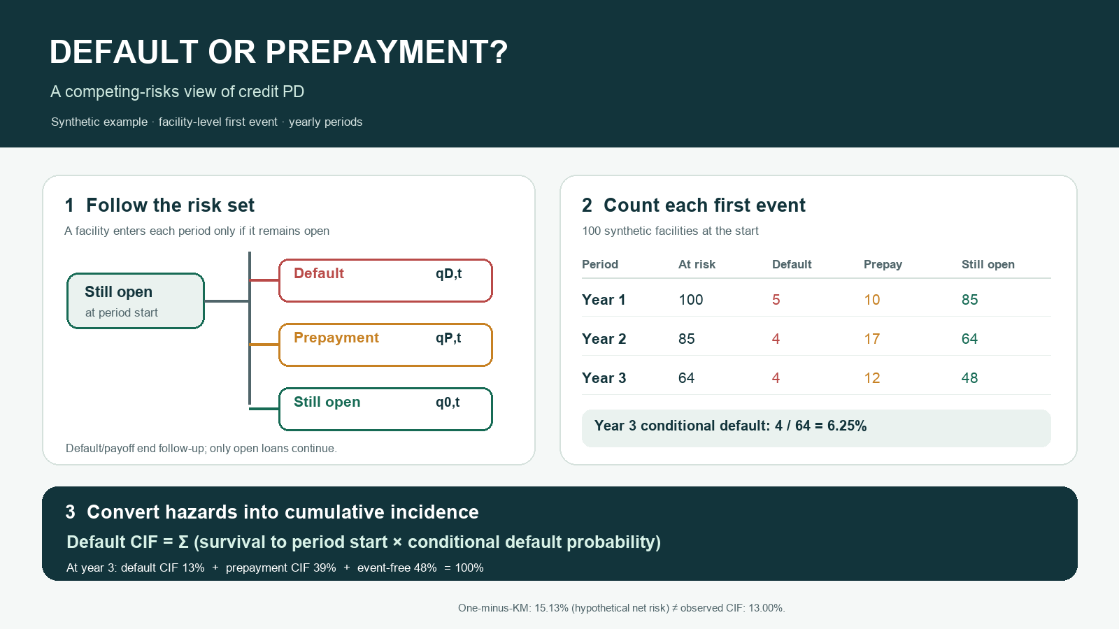
Year 1: 5 of 100 default and 10 prepay. Conditional default is 5/100 = 5%; default CIF is 100% × 5% = 5%.
Year 2: 85 remain. Conditional default is 4/85 = 4.71%. Its marginal probability from the original cohort is 85% × 4.71% = 4%; add this to 5%, giving a 9% default CIF. Prepayment CIF is 10% + 85% × 20% = 27%.
Year 3: conditional default is 4/64 = 6.25%; its marginal probability from the original cohort is 64% × 6.25% = 4%, so default CIF reaches 13%. Prepayment CIF is 39%, and 48% remain event-free: 13% + 39% + 48% = 100%.

COMPETING RISKS IN CREDIT PD: DEFAULT, PREPAYMENT, AND ACCOUNT CLOSURE

At a glance

When a loan can default or be prepaid, the first event may prevent the other from occurring for that facility. These are competing risks. If the question is “What is the probability this facility defaults by month 36 under its observed payoff process?”, estimate default cumulative incidence. Do not treat early payoff as ordinary censoring and report one minus Kaplan–Meier as the observed default probability. That answers a different hypothetical net-risk question.

1. Define the unit and terminal events

Define whether the analysis unit is a facility or an obligor. Full payoff may end facility-level follow-up, while an obligor who refinances with the same lender may remain in an obligor-level analysis.

Outcome — Definition — Effect on follow-up

Default — First occurrence of the documented default event — Event of interest; terminal

Prepayment — Full payoff before maturity and closure — Competing terminal event if exposure ends

Administrative censoring — Observation ends while the facility is open and event-free — Follow-up is incomplete; no event observed

Still exposed — Open and not in default at period end — Remains in next period’s risk set

Do not label an internal refinance, balance transfer, temporary cure, or data-feed gap as prepayment without checking the event definition. Recurrent defaults need an episode-level method; the example below is a first-event method.

2. Calculate conditional hazards and cumulative incidence

For discrete period t, nₜ is the number open and event-free at period start, dₜ defaults, and pₜ prepays. Each cause-specific hazard is conditional on still being event-free at the start of that period.

qD,t and qP,t are period-specific conditional probabilities, not lifetime PDs. Event-free survival through period t is:

The marginal probability mass for default during period t is the probability of reaching that period event-free times the conditional default probability:

Summing those marginal masses gives default cumulative incidence (CIF):

3. Worked example

100 synthetic facilities

All counts are illustrative and synthetic. Each row reconciles the event-free risk set.

Year 1 | 100 | 5 | 10 | 85 | 5.00% | 10.00% | 5.00% | 10.00% | 85.00%

Year 2 | 85 | 4 | 17 | 64 | 4.71% | 20.00% | 9.00% | 27.00% | 64.00%

Year 3 | 64 | 4 | 12 | 48 | 6.25% | 18.75% | 13.00% | 39.00% | 48.00%

Year-three conditional PD (6.25%) is not the same as the incremental default probability from the original cohort (4%), because only 64% reach year three still event-free.

4. Why censoring prepayment changes the question

A cause-specific model removes competing events from that cause’s risk set after they occur. It can describe default intensity among facilities still event-free. To predict observed real-world default CIF, combine the default process with other terminal-event hazards because prepayment changes how many facilities remain at risk.

Censoring prepayments in a one-minus-Kaplan–Meier calculation estimates a hypothetical net risk under assumptions; it does not generally estimate observed default incidence when competing events are present. For this toy cohort:

1 − (1 − 5/100) × (1 − 4/85) × (1 − 4/64) ≈ 15.13%

That differs from observed default CIF of 13%. These answer different questions. In real data, the difference depends on event definitions, follow-up, assumptions, and data.

5. Choose a method for the target

Aalen–Johansen / discrete CIF — Estimates observed event-specific cumulative incidence; useful as a cohort benchmark; handle administrative censoring correctly.

Cause-specific hazards — Models the event hazard among accounts still event-free; useful for drivers of event intensity; model relevant causes and combine with survival to predict CIF.

Fine–Gray subdistribution hazard — Directly models the CIF through a modified risk set; coefficients are not ordinary cause-specific hazard ratios.

Binary fixed-horizon label — Estimates default by a selected date; define early payoff treatment because simply dropping paid-off accounts changes the target.

No method is best for every question. Choose based on the target, data, and assumptions. Validate calibration and discrimination at the intended horizon.

6. Runnable Python

discrete competing-risk CIF

This deterministic example uses only built-ins and synthetic counts. It reads no files, accesses no network, and invokes no shell or system commands.

rows = [

{"period": "Year 1", "at_risk": 100, "default": 5, "prepay": 10},

{"period": "Year 2", "at_risk": 85, "default": 4, "prepay": 17},

{"period": "Year 3", "at_risk": 64, "default": 4, "prepay": 12},

]

survival = 1.0

default_cif = 0.0

prepay_cif = 0.0

net_default_survival = 1.0

for row in rows:

n = row["at_risk"]

q_default = row["default"] / n

q_prepay = row["prepay"] / n

if q_default + q_prepay > 1.0:

raise ValueError("Events exceed the risk set")

default_cif += survival * q_default

prepay_cif += survival * q_prepay

survival *= 1.0 - q_default - q_prepay

net_default_survival *= 1.0 - q_default

print(f"{row['period']}: default CIF={default_cif:.2%}, "

f"prepay CIF={prepay_cif:.2%}, event-free={survival:.2%}")

print(f"Final default CIF={default_cif:.2%}; prepayment CIF={prepay_cif:.2%}; "

f"event-free={survival:.2%}; one-minus-KM illustration="

f"{1.0 - net_default_survival:.2%}")

Expected final results: default CIF 13.00%, prepayment CIF 39.00%, event-free 48.00%, and one-minus-product-limit 15.13%. This example has no incomplete follow-up. For real data with administrative censoring and unequal follow-up, use an appropriate time-to-event estimator.

7. Monitor data and model performance

1. Freeze and version the analysis unit, index date, default and payoff definitions, horizon, cure/redefault treatment, maturity date, and facility-versus-obligor convention

2. Reconcile event capture to servicing and closure systems

Investigate duplicate events, impossible sequences, timestamp gaps, and unclassified closures.

3. Separate administrative right-censoring from competing prepayment; compare follow-up by product, vintage, score band, and calendar period

4. For mature cohorts and stated horizons, compare predicted with empirical default CIF by portfolio, segment, vintage, and score band

Report denominators, default and payoff counts, predicted and observed CIF, calibration difference, and uncertainty intervals.

5. Track both default and prepayment CIF, cause-specific hazards, event-free survival, and input drift

Lower default incidence may reflect higher early payoff rather than improved credit quality.

6. Test event definitions, out-of-time performance, time-varying effects, and whether modeled causes combine to reproduce the target CIF

Generic PSI or AUC thresholds do not replace CIF calibration.

8. Keep PD separate from accounting and capital

Internal risk management: choose the event, horizon, and payoff convention for the decision, then validate the resulting CIF.

IFRS 9 accounting: ECL is a probability-weighted present value of contractual cash shortfalls over the applicable horizon. Default CIF may be one model input; it is not itself the allowance.

Regulatory capital: prudential PD is subject to applicable Basel and local rules. The Basel IRB framework includes a long-run average of one-year default rates for applicable grades. This synthetic lifetime CIF is not a regulatory capital PD methodology.

Common mistakes

• Reporting one-minus-Kaplan–Meier with payoff censored as observed default incidence.

• Confusing a conditional yearly probability with cumulative lifetime PD.

• Predicting CIF from default hazard alone and ignoring payoff hazard.

• Failing to distinguish payoff from refinance, balance transfer, cure, or missing data.

• Interpreting Fine–Gray coefficients as ordinary cause-specific hazard ratios.

• Applying an uncensored toy calculation to incomplete follow-up.

References

Columbia University Mailman School of Public Health, Competing Risk Analysis: https://www.publichealth.columbia.edu/research/population-health-methods/competing-risk-analysis

Fine & Gray (1999), A Proportional Hazards Model for the Subdistribution of a Competing Risk: https://doi.org/10.1080/01621459.1999.10474144

Saavedra et al. (2024), Probability of default for lifetime credit loss for IFRS 9 using machine learning competing risks survival analysis models: https://doi.org/10.1016/j.eswa.2024.123607

IFRS Foundation, IFRS 9 Financial Instruments, B5.5.17 and B5.5.28–B5.5.29: https://www.ifrs.org/content/dam/ifrs/publications/pdf-standards/english/2022/issued/part-a/ifrs-9-financial-instruments.pdf?bypass=on

Basel Committee, Basel Framework CRE36: https://www.bis.org/basel_framework/standard/cre/36/inforce/2023-01-01/published/2022-12-08

Educational example only. Counts and rates are synthetic. Real implementation needs documented event definitions, data lineage, validation, and applicable accounting and prudential review.

Try a reproducible Python example

These examples use synthetic inputs and run locally in a browser worker. Edit the code, run it, and compare its output with the published example.

Runnable Python · local in your browser

Calculate WOE and IV from grouped counts

Use synthetic good and bad counts for three ordered scorecard bins. The 0.5 adjustment avoids a zero distribution in this small example.

Editable Python example

Output

Run the code to see the output.

Runtime loads only after you press Run. Code runs in a separate browser worker with a 10-second limit and a 20,000-character output cap. Use synthetic examples only; browser execution is not a secure environment for secrets or sensitive records.

Runnable Python · local in your browser

Convert a logistic model logit to PD

Apply the logistic function to an illustrative intercept plus two feature contributions.

Editable Python example

Output

Run the code to see the output.

Educational material only. Methods and examples are simplified; state and validate the assumptions required for your use case.