Credit scorecards

How to Calculate Predictor Weights in Logistic Regression: Coefficients, Contributions, and Scorecard Points

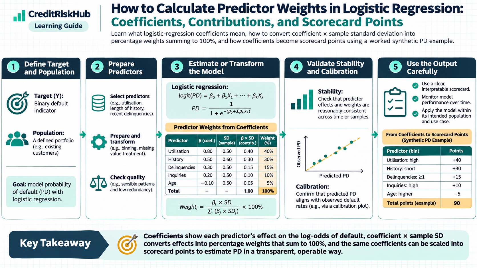
Learn what logistic-regression coefficients mean, how to convert coefficient × sample standard deviation into percentage weights summing to 100%, and how coefficients become scorecard points using a worked synthetic PD example.

Updated 2026-10-29

A visual overview of Learn what logistic-regression coefficients mean, how to convert coefficient × sample standard deviation into percentage weights summing to 100%, and how coefficients become scorecard points using a worked synthetic PD example. See the guide for assumptions and implementation details.

Purpose

Key terms

Hover over or focus a term for a quick definition, or open its glossary entry.

Formula

η = β₀ + β₁x₁ + β₂x₂ + ... + βₖxₖ
PD = p = 1 / (1 + exp(-η))
log(p / (1 - p)) = η
η = -3.20 + 0.18 × utilization_10pp + 0.95 × arrears_30dpd + (-0.04) × months_since_adverse_event
PD = 1 / (1 + exp(-η))
• Utilization: Code the percentage as ten-point units, so 70% becomes 7. Its coefficient is 0.18. Each additional 10 percentage points multiplies default odds by exp(0.18) ≈ 1.20, about a 20% increase, holding the other inputs fixed.
• Arrears indicator: Use 1 if the defined 30-DPD event occurred in the lookback, otherwise 0. Its coefficient is 0.95. Moving from 0 to 1 multiplies default odds by exp(0.95) ≈ 2.59, holding the other inputs fixed.
• Months since adverse event: Record the number of months, with zero meaning the event is current. Its coefficient is -0.04. Each additional month multiplies default odds by exp(-0.04) ≈ 0.961, about a 3.9% decrease, holding the other inputs fixed.

PURPOSE

People often ask for the “weight” of each independent variable in a credit-risk model. In logistic regression, the fitted coefficient is often called a weight, but it does not answer every question someone might mean by importance. A coefficient depends on the predictor’s units. A borrower-level contribution depends on that borrower’s predictor value. A scorecard point value also depends on the score scaling convention.

This guide separates those quantities, works through a synthetic probability-of-default (PD) model, and shows how the coefficients relate to odds, standardized effects, and points. The example is for learning; it is not a fitted or validated model.

THE LOGISTIC REGRESSION EQUATION

For a binary target where y = 1 means the defined default event occurred during the target horizon, a logistic regression model first calculates a linear predictor:

The model converts it to a probability using the logistic function:

Equivalently, the logit of the probability is the linear predictor:

Here, β₀ is the intercept, βⱼ is the coefficient for predictor j, and xⱼ is that predictor’s model input after any transformations, binning, or encoding. In scikit-learn, the fitted binary model exposes feature coefficients as coef_ and the intercept as intercept_; those coefficients belong to the model’s decision function. See the scikit-learn LogisticRegression reference (https://scikit-learn.org/stable/modules/generated/sklearn.linear_model.LogisticRegression.html).

WHAT “WEIGHT” CAN MEAN

Use the name that matches the quantity you calculate:

• Coefficient (βⱼ): change in log odds of the event for a one-unit increase in xⱼ, holding the model’s other included predictors fixed.

• Odds ratio (exp(βⱼ)): multiplier on the event odds for a one-unit increase in xⱼ, holding the other predictors fixed.

• Record-level contribution (βⱼxⱼ): the predictor’s contribution to a particular record’s linear predictor, given the model’s coding and reference point.

• Standardized coefficient (βⱼ × SD(xⱼ)): change in log odds for a one-standard-deviation increase in that predictor, with other predictors held fixed. This helps account for different units, but is not a universal feature-importance score.

• Normalized percentage weight: 100 × |βⱼ| × SD(xⱼ) / Σₖ(|βₖ| × SD(xₖ)), a descriptive allocation of absolute standardized-coefficient magnitudes across the included predictors. It sums to 100%, but is not a share of PD explained.

• Scorecard points: a scaled and often shifted or rounded transformation of the model’s predictor contributions. Points depend on the chosen score scale and odds convention.

A larger raw coefficient does not automatically mean a predictor is more important. One variable may be measured in dollars and another in thousands of dollars; simply changing units changes the coefficient while leaving predictions unchanged. Coefficients also describe a conditional relationship in the fitted model, not a causal effect.

WORKED EXAMPLE: A SYNTHETIC ONE-YEAR PD MODEL

Assume the target is whether a synthetic borrower defaults within the next twelve months, under a fixed, explicitly governed default definition. Suppose the fitted model is:

The inputs are defined as follows:

These are made-up coefficients and effects. They do not establish what relationships should appear in a real portfolio. In particular, the meaning of arrears_30dpd depends on how 30 DPD, the lookback, and the target default are defined.

CALCULATE ONE BORROWER’S PD

Consider a synthetic borrower with 70% utilization, the arrears indicator equal to 1, and zero months since the adverse event. The linear-predictor contributions are:

• Intercept: -3.20.

• Utilization: 0.18 × 7 = +1.26.

• Arrears indicator: 0.95 × 1 = +0.95.

• Months since event: -0.04 × 0 = 0.00.

• Total logit: -3.20 + 1.26 + 0.95 + 0.00 = -0.99.

Convert the total to probability:

PD = 1 / (1 + exp(0.99)) ≈ 0.271, or about 27.1%.

The coefficient is not the same as the borrower’s contribution. The arrears coefficient is 0.95; for this borrower its contribution is 0.95 × 1 = 0.95. If the indicator were zero, its contribution would be zero, but the model’s coefficient would remain 0.95.

For a borrower-specific percentage summary, first calculate each predictor contribution cⱼ = βⱼxⱼ (or βⱼ(xⱼ - referenceⱼ) when explaining a change from an explicit baseline). One transparent convention is to report each predictor’s share of the absolute predictor contributions, excluding the intercept:

local shareⱼ (%) = 100 × |cⱼ| / Σₖ|cₖ|

For this borrower, the denominator is |1.26| + |0.95| + |0.00| = 2.21. Utilization contributes 1.26 / 2.21 = 57.0% of the absolute predictor contribution; the arrears flag contributes 0.95 / 2.21 = 43.0%; months since event contributes 0.0%. These percentages sum to 100% because they describe relative magnitudes. Keep the signed contributions beside them: utilization and arrears each increase this model’s default log odds, while a negative signed contribution would reduce it. If all predictor contributions are zero, the percentage is undefined.

This is a local, borrower-specific percentage summary, not a universal variable-importance measure. Excluding the intercept is deliberate: the intercept is the model baseline, not an input variable. For a portfolio-level descriptive summary, choose and document a reference value for each input, calculate Aⱼ = averageᵢ(|βⱼ(xᵢⱼ - referenceⱼ)|) on a named sample, and report 100 × Aⱼ / ΣₖAₖ. The reference point and sample mix affect the result, so use the same definitions and population when comparing periods. Neither percentage proves causality or unique importance, particularly when predictors are correlated.

At 70% utilization with no arrears flag, the model gives η = -1.94 and PD of about 12.6%. Turning the arrears flag on adds 0.95 to log odds and multiplies odds by about 2.59; it does not multiply the probability by 2.59. The resulting PD is about 27.1%. This distinction matters because logistic effects are linear in log odds, not in probability.

WHY COEFFICIENT SIZE DEPENDS ON UNITS

In the example, utilization is expressed in ten-percentage-point units, so a ten-point rise has coefficient 0.18. If utilization were instead entered as a percentage-point value from 0 to 100, the equivalent coefficient would be 0.018. If entered as a fraction from 0 to 1, the equivalent coefficient would be 1.8. All three parameterizations can produce the same predictions when coefficients are transformed consistently.

For a continuous variable with coefficient β, multiplying the predictor by a constant c requires dividing its coefficient by c to preserve the linear predictor. Therefore, do not rank predictors by absolute raw coefficients unless their units and codings are directly comparable.

COMPARE EFFECTS USING STANDARD DEVIATIONS

A common descriptive comparison is the standardized coefficient βⱼ × SD(xⱼ). For illustration, suppose the model-development sample has these synthetic standard deviations:

• Utilization in ten-point units: coefficient 0.18; sample standard deviation 2.0; standardized coefficient 0.18 × 2.0 = 0.36.

• 30-DPD indicator with 10% event prevalence: coefficient 0.95; standard deviation sqrt(0.10 × 0.90) = 0.30; standardized coefficient 0.95 × 0.30 = 0.285.

• Months since event: coefficient -0.04; sample standard deviation 6.0 months; standardized coefficient -0.04 × 6.0 = -0.24.

These values describe conditional changes in log odds associated with a one-standard-deviation change in each input, under this fitted model. They are more scale-aware than raw coefficients, but still depend on the sample distribution and model specification. For a binary predictor, its standard deviation changes with the event prevalence. Correlated predictors can also split or redistribute fitted effects, so standardized coefficients are not a stand-alone ranking of causal or unique importance.

EXPRESS STANDARDIZED EFFECTS AS PERCENTAGES THAT SUM TO 100%

If you need a simple model-level percentage allocation across predictors, define the magnitude for predictor j as its absolute standardized coefficient:

aⱼ = |βⱼ| × SD(xⱼ)

Then normalize those magnitudes across the k included predictors:

weightⱼ (%) = 100 × aⱼ / Σₖ aₖ = 100 × |βⱼ| × SD(xⱼ) / Σₖ(|βₖ| × SD(xₖ))

Using the synthetic development-sample values above:

• Utilization: |0.18| × 2.0 = 0.360; percentage weight 100 × 0.360 / 0.885 = 40.7%.

• 30-DPD indicator: |0.95| × 0.30 = 0.285; percentage weight 100 × 0.285 / 0.885 = 32.2%.

• Months since event: |-0.04| × 6.0 = 0.240; percentage weight 100 × 0.240 / 0.885 = 27.1%.

• Total: 0.360 + 0.285 + 0.240 = 0.885; rounded percentage weights sum to 100.0%.

Keep the signed standardized coefficients beside these percentages: utilization +0.360, 30-DPD +0.285, and months since event −0.240. The sign shows direction; the percentage formula uses absolute values so that opposing effects do not cancel and all shares can sum to 100%.

Call this a normalized absolute standardized-coefficient share, and state the sample used to calculate each standard deviation. It is a convenient descriptive comparison, not a percentage of PD, defaults, or model accuracy explained by a variable. It does not establish causality or unique predictive importance. Shares depend on the sample distribution, transformations, model specification, and correlated predictors; binary-variable SD also depends on prevalence. For a different question—how much the predictors contribute for one borrower—use the local contribution method above. For predictive reliance, assess out-of-time metric changes with carefully designed ablation or permutation analyses.

Use an out-of-time validation cohort to evaluate whether a model predicts well. For predictor-level reliance, consider carefully designed ablation or permutation comparisons, grouped when variables are correlated, and measure the change in relevant out-of-time metrics. Such measures answer predictive reliance questions, not causality. Check coefficient signs, uncertainty, stability across vintages, and sensitivity to alternative reasonable model specifications.

WHEN PREDICTORS ARE BINNED AND TRANSFORMED TO WOE

Traditional scorecards often bin a raw predictor and replace its value with the bin’s Weight of Evidence (WOE). The model then uses WOEⱼ, not the original raw value:

η = β₀ + β₁WOE₁ + β₂WOE₂ + ... + βₖWOEₖ

In that case, βⱼ is the coefficient per one-unit change in the encoded WOE input. The WOE value summarizes the good-versus-bad distribution for a bin under the chosen convention; the regression coefficient then combines that encoded variable with the other model predictors. If the definition uses ln(good share / bad share), the WOE sign has the opposite orientation from a convention using ln(bad share / good share). State the convention and verify the resulting sign and risk ordering.

A coefficient alone does not give the points for a bin. The bin’s unscaled model contribution is βⱼ × WOEⱼ. A scorecard then applies a chosen shift and slope, and may allocate the intercept across predictor point tables or report base points separately. MathWorks documents this score construction as a shifted and scaled combination of the intercept, model coefficients, and WOE values in its scorecard points and scaling reference (https://www.mathworks.com/help/finance/creditscorecard.formatpoints.html).

CONVERT COEFFICIENTS TO SCORECARD POINTS

For a score that increases as risk decreases, let the model’s default log odds be η, and define:

Score = A - B × η

If the score scale uses PDO points to double the good-to-bad odds, then a common slope magnitude is:

B = PDO / ln(2)

For example, with PDO = 20, B = 20 / ln(2) ≈ 28.85. The utilization coefficient of 0.18 means each additional 10 percentage points lowers the score by approximately 28.85 × 0.18 = 5.19 points, before any rounding or binning. The 30-DPD coefficient of 0.95 means changing the flag from 0 to 1 lowers the score by approximately 28.85 × 0.95 = 27.41 points. A negative coefficient reverses the direction and increases the score as the input increases.

A determines the score offset and is selected to place a chosen reference odds at a chosen score. A production scorecard must define the bad/good event orientation, base odds, base score, PDO, binning, WOE sign convention, missing-value treatment, and rounding rule. If the event or sign convention changes, the point direction can change. Validate that summing the point contributions and base points reproduces the model’s intended log odds and PD after scaling.

PRACTICAL WORKFLOW

• Define the target event, prediction date, performance horizon, eligible population, and event maturity before fitting the model.

• Document each predictor’s unit, reference value, transformation, binning, missing-value rule, and direction.

• Fit the model using training data only; freeze preprocessing and coefficient versions together.

• Report coefficients with standard errors or uncertainty intervals, odds ratios, and the input-unit interpretation. Avoid calling absolute coefficients a universal importance measure.

• For individual explanations, show each βⱼxⱼ contribution to the logit and identify the intercept or reference baseline.

• If comparing predictor scale effects, report βⱼ × SD(xⱼ) with the sample and period used to calculate each SD, and explain limitations for binary and correlated inputs.

• For scorecards, convert contributions using an explicit score scale and test score-to-odds-to-PD consistency.

• Validate discrimination, calibration, stability, data quality, and outcomes on representative out-of-time data. A stable sign or high absolute coefficient is not proof that a predictor is safe, causal, fair, or useful.

LIMITATIONS AND INTERPRETATION

• The numerical example uses synthetic data and invented coefficients; it is not suitable for an application or portfolio decision.

• Logistic coefficients describe conditional association within the selected model and dataset. They do not prove causation.

• Odds ratios are not probability ratios. A fixed coefficient can correspond to very different probability changes at different baseline PD levels.

• Standardized coefficients depend on the sample standard deviations; for binary and categorical predictors, comparisons need particular care.

• Correlation, regularization, omitted predictors, interactions, nonlinearities, and sample selection can all affect coefficients and signs.

• A coefficient or scorecard point table does not, by itself, establish calibration, fair treatment, regulatory acceptability, or IFRS 9 compliance.

• An internal score, a regulatory-capital PD, and an IFRS 9 accounting ECL estimate serve different purposes. A logistic PD component is not by itself a complete ECL calculation.

REFERENCES

• scikit-learn, LogisticRegression API reference (https://scikit-learn.org/stable/modules/generated/sklearn.linear_model.LogisticRegression.html), including its coefficient, intercept, and probability prediction attributes.

• MathWorks, Format scorecard points and scaling (https://www.mathworks.com/help/finance/creditscorecard.formatpoints.html), including the coefficient × WOE construction and shift/slope score scaling.

• MathWorks, About Credit Scorecards (https://www.mathworks.com/help/finance/about-credit-scorecards.html), explaining how binned attributes, WOE, logistic coefficients, and scorecard points fit together.

Educational material only. Validate model interpretation and score scaling under the institution’s approved model-development and governance standards before operational use.

Try a reproducible Python example

These examples use synthetic inputs and run locally in a browser worker. Edit the code, run it, and compare its output with the published example.

Runnable Python · local in your browser

Calculate WOE and IV from grouped counts

Use synthetic good and bad counts for three ordered scorecard bins. The 0.5 adjustment avoids a zero distribution in this small example.

Editable Python example

Output

Run the code to see the output.

Runtime loads only after you press Run. Code runs in a separate browser worker with a 10-second limit and a 20,000-character output cap. Use synthetic examples only; browser execution is not a secure environment for secrets or sensitive records.

References

scikit-learn and MathWorks documentation — scikit-learn and MathWorks documentation

Educational material only. Methods and examples are simplified; state and validate the assumptions required for your use case.