Probability of default (PD)
PD Segmentation (3/3): Python Implementation and Validation Tests
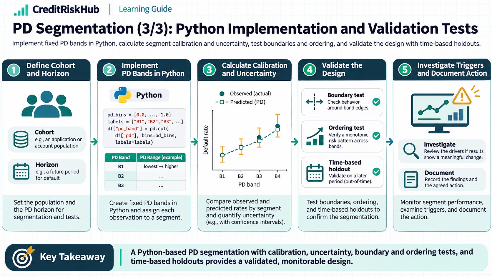
Implement fixed PD bands in Python, calculate segment calibration and uncertainty, test boundaries and ordering, and validate the design with time-based holdouts.
Updated 2026-10-25
Purpose
Implement fixed PD bands in Python, calculate segment calibration and uncertainty, test boundaries and ordering, and validate the design with time-based holdouts.
Key terms
Hover over or focus a term for a quick definition, or open its glossary entry.
European Banking Authority, Guidelines on PD estimation, LGD estimation and treatment of defaulted assets (EBA/GL/2017/16; applicable to its defined EU IRB scope): https://eba.europa.eu/activities/single-rule-book/regulatory-activities/model-validation/guidelines-pd-estimation-lgd?version=2018PD SEGMENTATION SERIES — PART 3 OF 3
IMPLEMENTING AND TESTING PD SEGMENTS WITH PYTHON
This guide turns a segmentation design into reproducible assignment rules and validation checks. The example uses a fixed set of synthetic, matured one-year outcomes and only Python’s standard library. It demonstrates segment-level observed-versus-expected analysis and basic tests; its tiny samples are for teaching, not production calibration.
TEST THE DESIGN AT FOUR LEVELS
1. Data and target tests
Validate unique keys, allowed default labels (0/1), PD range [0,1], reporting dates, missing values, duplicates, and outcome maturity. Verify that every record belongs to the intended portfolio and every prediction uses only information available at its forecast date. Preserve exclusions and their reasons.
2. Assignment tests
Apply the frozen cutoffs or rules to known boundary cases. Check that every eligible account is assigned exactly once, no ineligible account is accidentally scored, unknown values have explicit handling, and rule versions match the model version. Test cutoffs immediately below, at, and above each boundary. Test whether an assigned grade can change because of a data-type or category-mapping issue.
3. Statistical validation
On a time-based holdout with matured outcomes, compare segment size, default count, mean predicted PD, observed default rate, O/E, and uncertainty. Check risk ordering if ordered grades are intended. Test whether within-segment risk variation is acceptable for the use, while recognizing low-default uncertainty. A good in-sample split is not enough: rules learned from future data leak outcome information.
4. Operational and governance tests
Reconcile output counts and exposures to the source; compare production and independent implementations on a sample; verify logging, approvals, exception pathways, versioning, and rollback. Re-run the same input snapshot and confirm the same assignments and metrics. Document changes to cutoffs and monitor them as model changes.
SYNTHETIC EXAMPLE AND FIXED RULE
We illustrate three PD bands using thresholds 5% and 20%: Low below 5%, Medium from 5% to below 20%, and High at 20% or above. These cutoffs are invented for demonstration; they are not recommended thresholds. There are four observations per segment. Observed defaults are 0/4, 1/4, and 2/4 respectively. Because the groups are tiny, their confidence intervals are very wide. The example can test code and expected behavior, but cannot support a credible business conclusion.
COPY AND RUN: SEGMENT METRICS AND GUARDRAIL TESTS
The following Python 3 code assigns segments from PD, checks boundary behavior and data validity, then reports observed rates, mean PD, O/E, and Wilson 95% intervals. It uses 12 fixed synthetic records, performs no network or file access, and has bounded execution.
from math import sqrt
records = [
{"id": "L1", "pd": 0.02, "default": 0},
{"id": "L2", "pd": 0.02, "default": 0},
{"id": "L3", "pd": 0.02, "default": 0},
{"id": "L4", "pd": 0.02, "default": 0},
{"id": "M1", "pd": 0.10, "default": 0},
{"id": "M2", "pd": 0.10, "default": 1},
{"id": "M3", "pd": 0.10, "default": 0},
{"id": "M4", "pd": 0.10, "default": 0},
{"id": "H1", "pd": 0.30, "default": 1},
{"id": "H2", "pd": 0.30, "default": 0},
{"id": "H3", "pd": 0.30, "default": 1},
{"id": "H4", "pd": 0.30, "default": 0},
]
order = ["Low", "Medium", "High"]
def assign_segment(pd):
if pd < 0.05:
return "Low"
if pd < 0.20:
return "Medium"
return "High"
def wilson_interval(defaults, n, z=1.96):
rate = defaults / n
denominator = 1 + z * z / n
center = (rate + z * z / (2 * n)) / denominator
margin = z * sqrt(rate * (1 - rate) / n + z * z / (4 * n * n)) / denominator
return max(0.0, center - margin), min(1.0, center + margin)
assert len({row["id"] for row in records}) == len(records)
assert all(row["default"] in (0, 1) for row in records)
assert all(0.0 <= row["pd"] <= 1.0 for row in records)
assert [assign_segment(x) for x in (0.049, 0.05, 0.199, 0.20)] == ["Low", "Medium", "Medium", "High"]
for row in records:
row["segment"] = assign_segment(row["pd"])
summary = []
for segment in order:
group = [row for row in records if row["segment"] == segment]
n = len(group)
defaults = sum(row["default"] for row in group)
expected = sum(row["pd"] for row in group)
observed_rate = defaults / n
mean_pd = expected / n
lower, upper = wilson_interval(defaults, n)
summary.append((segment, n, defaults, mean_pd, observed_rate, defaults / expected, lower, upper))
assert sum(row["segment"] in order for row in records) == len(records)
assert all(summary[i][4] <= summary[i + 1][4] for i in range(len(summary) - 1))
for segment, n, defaults, mean_pd, observed_rate, oe, lower, upper in summary:
print(f"{segment}: n={n}, defaults={defaults}, mean PD={mean_pd:.3f}, ODR={observed_rate:.3f}, O/E={oe:.2f}, Wilson95=({lower:.3f}, {upper:.3f})")
Expected output should show rates of 0%, 25%, and 50%, increasing across these illustrative bands. The assertions test the declared rule, valid values, unique IDs, complete assignment, and this example’s ordering. They do not prove that the thresholds generalize, that the PD model is calibrated, or that differences are statistically significant. Wilson intervals assume independent Bernoulli outcomes; clustered borrowers, weighting, censoring, or portfolio selection may require other methods.
HOW TO TEST ON REAL DEVELOPMENT DATA
Use chronological development, validation, and out-of-time periods. Make the observation window long enough for the target horizon to mature, and label incomplete windows. If a borrower appears more than once, split by borrower or use a design that accounts for dependence. Choose cutoffs and model complexity using development data only; use a separate validation set to compare alternatives, and keep the final out-of-time window untouched until design choices are fixed.
For each segment report n, defaults, exposure, mean PD, observed rate, confidence interval, and O/E. Evaluate calibration by segment and relevant subgroups; discrimination using suitable ranking measures; stability of population and assignment; and operational complexity. Compare a proposed split with the parent segment: does it improve decision-relevant differentiation enough to justify added variance, monitoring burden, and governance? Avoid selecting cutoffs just because they create a monotonic chart on one sample.
When defaults are rare, uncertainty dominates. Pool adjacent groups, use a longer representative history, compare external or benchmark data where appropriate, and report uncertainty. Any shrinkage or smoothing must be explicit and validated. A zero observed default count does not imply zero true PD. If testing many candidate splits, account for the selection process rather than treating the best-looking in-sample split as an unbiased result.
MONITOR THE TESTED VERSION
Store code, data snapshot identifiers, cutoff definitions, feature transformations, default definition, sample dates, outputs, and approvals. In production, monitor assignment drift, segment sizes, migration, missing or unknown categories, and matured calibration. Retest after changes to policy, data, score, population, or outcome definition. A production test should fail visibly when an account is unassigned, appears in multiple mutually exclusive bands, or is evaluated against an immature target window.
MEASURE BOUNDARIES
The sample code measures a simple one-year default outcome. It is not an IFRS 9 lifetime ECL calculation and does not estimate Basel capital. Basel IRB requirements apply to their defined banking scope and include rating-system design, assignment, estimation, and validation expectations. Internal risk measures should be governed for their own purposes. Do not present a statistical test as automatic evidence of compliance.
REFERENCES
Basel Framework, CRE 36 — IRB minimum requirements, including rating-system design, out-of-time/out-of-sample validation, PD estimation, and ongoing requirements for banks in scope: https://www.bis.org/committees/bcbs/basel-framework/standard/cre/36/inforce/2023-01-01/published/2020-03-27
Educational example only. Thresholds, records, and defaults are synthetic. Validate definitions, sample design, statistical assumptions, and regulatory applicability before operational use.
Try a reproducible Python example
These examples use synthetic inputs and run locally in a browser worker. Edit the code, run it, and compare its output with the published example.
Runnable Python · local in your browser
Convert a logistic model logit to PD
Apply the logistic function to an illustrative intercept plus two feature contributions.
Output
Run the code to see the output.
Runtime loads only after you press Run. Code runs in a separate browser worker with a 10-second limit and a 20,000-character output cap. Use synthetic examples only; browser execution is not a secure environment for secrets or sensitive records.
Runnable Python · local in your browser
Calculate year-by-year marginal and cumulative PD
Follow years 1–3 separately: conditional PD is the rate among survivors, marginal PD is the share of the original cohort defaulting in that year, and cumulative PD adds those marginal shares.
Output
Run the code to see the output.
Runtime loads only after you press Run. Code runs in a separate browser worker with a 10-second limit and a 20,000-character output cap. Use synthetic examples only; browser execution is not a secure environment for secrets or sensitive records.
References
- Basel Committee on Banking Supervision; European Banking Authority — Basel Committee on Banking Supervision; European Banking Authority
Educational material only. Methods and examples are simplified; state and validate the assumptions required for your use case.