Probability of default (PD)
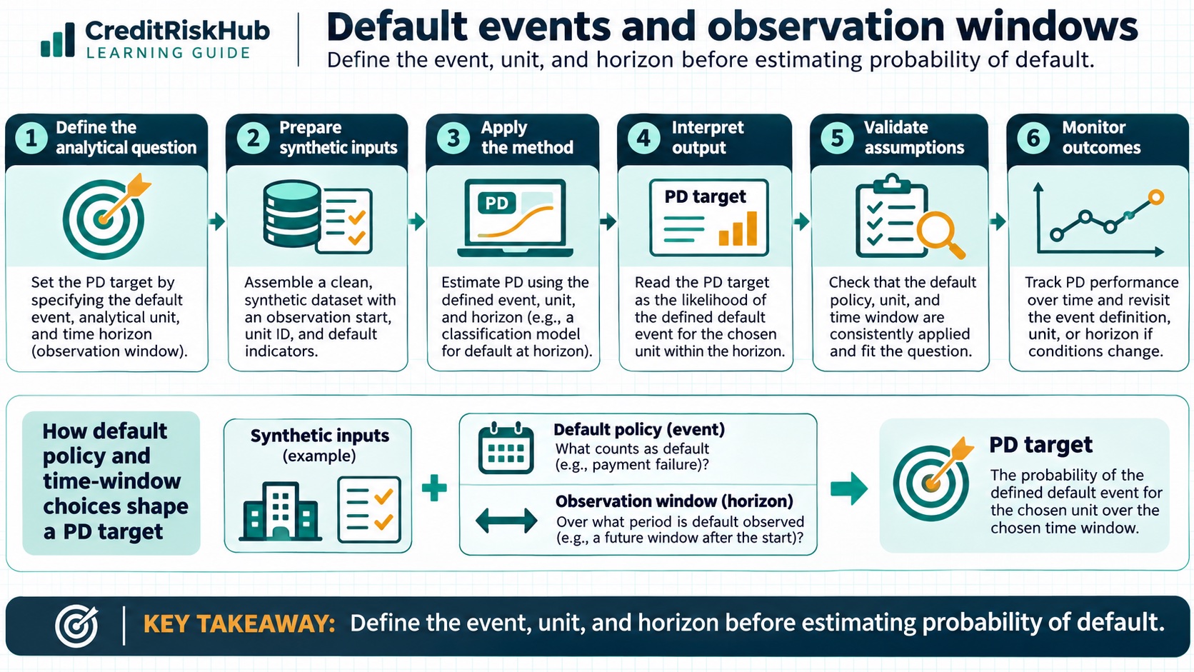
Default events and observation windows
Define the event, unit, and horizon before estimating probability of default.
Purpose
Show how default policy and time-window choices shape a PD target.
Key terms
Hover over or focus a term for a quick definition, or open its glossary entry.
Key definitions
- PD is the probability of a defined default event occurring for a defined exposure or obligor over a specified horizon.
- An observation window supplies predictors; a performance window determines when the target is observed.
Observed one-year default rate = unique defaults during the next 12 months ÷ eligible non-defaulted units at start.Worked example
With 28 defaults among 2,000 eligible obligors followed for a full year, the raw rate is 1.4%.
Detailed explanation
The target definition is a modeling decision with policy consequences. Specify which events count as default, whether the unit is an obligor or facility, how cure and re-default are handled, and the date at which eligibility is measured. If the target window is 12 months, every included account must either be observed for the full window or handled with a defensible censoring method.
Avoid using information generated after the observation date. Record definition changes and reconcile the target to relevant business and regulatory standards. A Basel reference definition helps explain prudential IRB conventions, but it does not automatically define the accounting default assessment or every lender's internal decision target.
Try a reproducible Python example
These examples use synthetic inputs and run locally in a browser worker. Edit the code, run it, and compare its output with the published example.
Runnable Python · local in your browser
Convert a logistic model logit to PD
Apply the logistic function to an illustrative intercept plus two feature contributions.
Output
Run the code to see the output.
Runtime loads only after you press Run. Code runs in a separate browser worker with a 10-second limit and a 20,000-character output cap. Use synthetic examples only; browser execution is not a secure environment for secrets or sensitive records.
Runnable Python · local in your browser
Calculate year-by-year marginal and cumulative PD
Follow years 1–3 separately: conditional PD is the rate among survivors, marginal PD is the share of the original cohort defaulting in that year, and cumulative PD adds those marginal shares.
Output
Run the code to see the output.
Runtime loads only after you press Run. Code runs in a separate browser worker with a 10-second limit and a 20,000-character output cap. Use synthetic examples only; browser execution is not a secure environment for secrets or sensitive records.
Assumptions
- Defaults are assigned consistently and each record has enough follow-up for its target horizon.
Limitations
- Censoring and competing exits can bias a simple count.
- Basel regulatory default definitions are purpose-specific and should not be silently substituted for accounting policy.
References
- Basel Framework: IRB approach and credit-risk components — Basel Committee on Banking Supervision
- Guidance on credit risk and accounting for expected credit losses — Basel Committee on Banking Supervision
Educational material only. Methods and examples are simplified; state and validate the assumptions required for your use case.