Probability of default (PD)
PD Segmentation (2/3): Monitoring Calibration, Drift, and Migration
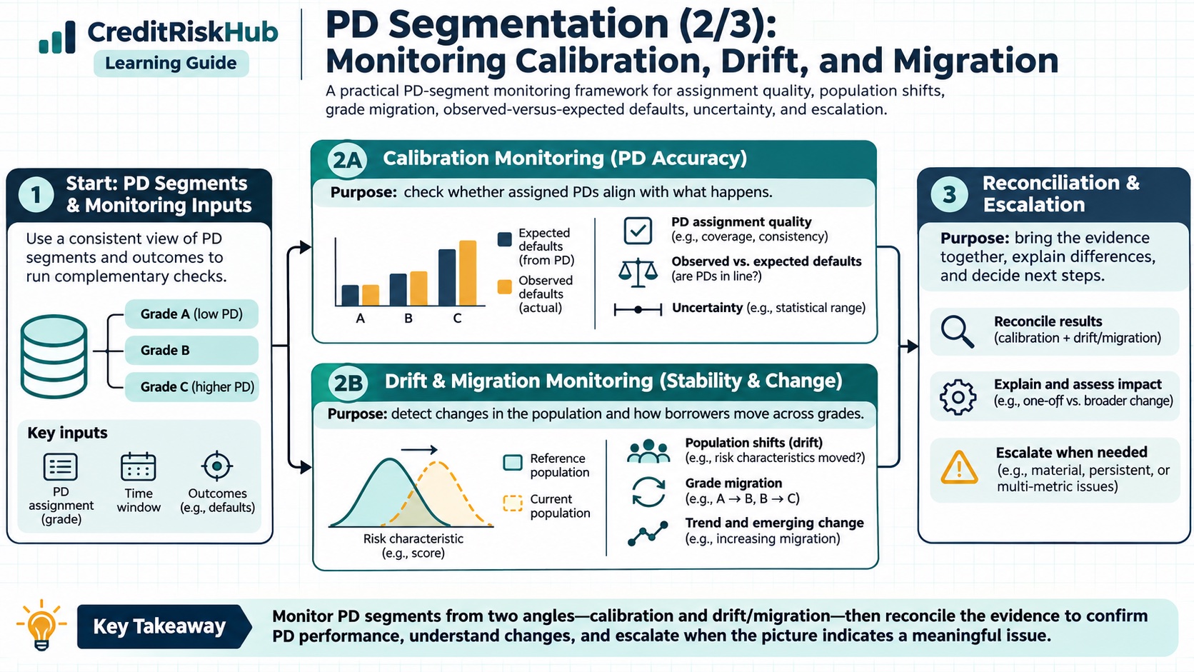
A practical PD-segment monitoring framework for assignment quality, population shifts, grade migration, observed-versus-expected defaults, uncertainty, and escalation.
Updated 2026-10-25
Purpose
A practical PD-segment monitoring framework for assignment quality, population shifts, grade migration, observed-versus-expected defaults, uncertainty, and escalation.
Key terms
Hover over or focus a term for a quick definition, or open its glossary entry.
European Banking Authority, EBA/GL/2017/16 — PD and LGD estimation guidelines; see the sections on rating assignment, calibration, and estimation data for the defined EU IRB context: https://eba.europa.eu/activities/single-rule-book/regulatory-activities/model-validation/guidelines-pd-estimation-lgd?version=2018PD SEGMENTATION SERIES — PART 2 OF 3
MONITORING PD SEGMENTS OVER TIME
A segmentation remains useful only while its assignment rules, data, and estimated risk stay fit for their intended use. Monitoring should answer three separate questions: are accounts still assigned correctly; has the population changed; and do matured outcomes remain consistent with the PDs? Looking only at portfolio-wide default rate can hide a failing segment behind a stable average.
Start by fixing the unit (obligor or facility), default definition, forecast horizon, reporting date, population perimeter, and outcome-maturity rule. A one-year forecast should be compared with a fully observed one-year outcome window, or explicitly marked immature/censored. Do not treat loans with incomplete follow-up as non-defaults. If repeated observations are used, define weights and prevent repeated borrowers from distorting counts.
THE MONITORING LAYERS
1. Data and assignment controls
By segment and period, report record counts, unique obligors, exposure, missing/unmapped rates, invalid PD values, category changes, assignment failures, and rule/model version. Reconcile segment totals to the source portfolio. Track overrides, manual movement, and changes in score cutoffs.
2. Population mix
Monitor each segment’s share by obligor and exposure, plus product, geography, vintage, channel, rating, and key feature distributions. A simple segment-share shift is current share minus reference share. PSI can summarize changes across fixed bins: PSI = Σ (current share − reference share) × ln(current share / reference share). Handle zero shares with a documented smoothing convention. PSI is a screening statistic: it does not prove calibration deterioration and has no universal alert cutoff. Keep bins and reference period fixed for comparability.
3. Migration and transitions
Count movements between grades or pools from one date to the next. Report upgrades, downgrades, exits, new originations, and changes caused by model or policy versions separately. A transition matrix can reveal drift or operational churn that a one-date mix misses. When comparing cohorts, distinguish migration of existing obligors from changing origination mix.
4. Calibration by segment
For a matured cohort of n accounts, observed default rate (ODR) = D / n. Expected defaults = Σ PDᵢ. Observed-to-expected (O/E) = D / Σ PDᵢ. O/E above one means observed defaults exceed the model’s expected count in that sample; below one means fewer defaults occurred. Always display D, n, expected count, horizon, and the ODR alongside the ratio. Small denominators make O/E volatile.
Compare observed rate with mean predicted PD by segment and by relevant subgroups such as vintage, product, geography, or score band. A calibration plot and confidence interval are more informative than a single pass/fail flag. Check ranking separately: AUC or rank-order tests can show whether higher-risk groups rank worse, but a good ranking does not establish accurate PD levels. Conversely, recalibration can correct levels without fixing poor ordering.
5. Stability and risk context
Compare changes with economic conditions, underwriting policy, collections, portfolio growth, and data capture. For PIT PD, changes may be expected as current conditions change. For TTC PD, cyclical changes may be dampened by design, but the score distribution, long-run calibration, and grade migration still need review. State the model concept before interpreting movement.
WORKED SYNTHETIC EXAMPLE
A fixed segment has 400 matured one-year accounts, 16 observed defaults, and a sum of forecasts of 12 expected defaults. ODR = 16/400 = 4%; O/E = 16/12 = 1.33. A Wilson 95% interval for the observed rate is approximately 2.5% to 6.4%. Because the forecasted 3% lies within that broad interval, the sample alone gives limited evidence of a statistically clear difference. It is a monitoring signal: check adjacent periods, segment mix, economic context, and the calibration sample before deciding whether action is needed. This example is synthetic and the interval is an approximate binomial interval; it does not resolve dependence, weighting, or portfolio-design issues.
A practical table might show: Period | Segment | Matured n | Defaults | Mean PD | ODR | O/E | ODR interval | exposure share | unmapped %. Include an overall row and stable comparison periods. If the segment was created or redefined mid-period, do not present the resulting discontinuity as pure risk drift.
ESCALATION AND ACTIONS
Set investigation triggers through model purpose, materiality, default frequency, exposure, and risk appetite. Do not adopt a borrowed PSI, O/E, or minimum-default cutoff as if it were universal. When a trigger fires: first verify labels, maturity, joins, population, weights, and the version of segment rules; then identify which features and subgroups drove the change; compare observed and predicted outcomes with uncertainty; consider benchmarking or a challenger; and document the proposed action, owner, approval, and follow-up date.
Possible responses include correcting a data pipeline, reviewing a mapping, recalibrating PD levels, revising a segment boundary, gathering more evidence, applying an approved override, or restricting use. A metric crossing a threshold is an investigation trigger, not an automatic instruction to alter a model. Assess customer and business effects before changing eligibility, pricing, or credit decisions.
ACCOUNTING AND REGULATORY BOUNDARIES
An internal monitoring report, an IFRS 9 ECL estimate, and Basel IRB PD validation can share data but have different objectives and rules. IFRS 9 requires accounting measurement under the reporting entity’s applicable standards and forward-looking assumptions; Basel IRB requirements apply to banks and exposures in their prudential scope; internal monitoring thresholds should match their approved use. A one-year observed default rate is not by itself a lifetime ECL backtest or a regulatory capital result.
REFERENCES
Basel Framework, CRE 36 — IRB approach minimum requirements (rating assignment, validation, PD estimation; applicability is limited to its prudential scope): https://www.bis.org/committees/bcbs/basel-framework/standard/cre/36/inforce/2023-01-01/published/2020-03-27
NEXT IN THIS SERIES
Part 3 shows how to calculate segment-level calibration metrics in Python and test assignment, ordering, and time-based performance using synthetic outcomes.
Educational guide only. Use matured, correctly defined outcomes and portfolio-specific governance. The example is synthetic and is not regulatory advice.
Try a reproducible Python example
These examples use synthetic inputs and run locally in a browser worker. Edit the code, run it, and compare its output with the published example.
Runnable Python · local in your browser
Convert a logistic model logit to PD
Apply the logistic function to an illustrative intercept plus two feature contributions.
Output
Run the code to see the output.
Runtime loads only after you press Run. Code runs in a separate browser worker with a 10-second limit and a 20,000-character output cap. Use synthetic examples only; browser execution is not a secure environment for secrets or sensitive records.
Runnable Python · local in your browser
Calculate year-by-year marginal and cumulative PD
Follow years 1–3 separately: conditional PD is the rate among survivors, marginal PD is the share of the original cohort defaulting in that year, and cumulative PD adds those marginal shares.
Output
Run the code to see the output.
Runtime loads only after you press Run. Code runs in a separate browser worker with a 10-second limit and a 20,000-character output cap. Use synthetic examples only; browser execution is not a secure environment for secrets or sensitive records.
References
- Basel Committee on Banking Supervision; European Banking Authority — Basel Committee on Banking Supervision; European Banking Authority
Educational material only. Methods and examples are simplified; state and validate the assumptions required for your use case.