PD Segmentation (1/3): Common Methods and How to Choose

PD segmentation divides borrowers or exposures into groups that are similar enough for risk measurement and useful enough for decisions. A segment should capture meaningful differences in defaultA defined credit event used for measurement; the exact triggers depend on the applicable accounting, regulatory, or internal policy.Open full glossary entry ↗ risk while retaining enough comparable observations to estimate and monitor that risk. For banks using the Basel IRB framework, rating systems must meaningfully differentiate risk and support reasonably accurate, consistent estimates; retail pools are expected to be sufficiently homogeneous. These are prudential requirements for their applicable scope, not universal rules for every internal or accounting model.

Before choosing an algorithm, state the use: underwriting, pricing, portfolioA defined group of credit exposures analyzed together under stated inclusion rules.Open full glossary entry ↗ monitoring, IFRS 9The International Financial Reporting Standard for financial instruments, including classification, measurement, hedge accounting, and impairment requirements.Open full glossary entry ↗ input, internal risk appetiteThe amount and types of risk an organization is prepared to accept while pursuing its objectives.Open full glossary entry ↗, or regulatory estimation. Define the target default event, observation unit, forecast horizon, reference population, and whether the PD is point-in-time (PIT) or through-the-cycle (TTC). A segment built for a one-year consumer-loan decision may not suit a lifetime accounting estimate or a corporate IRB grade.

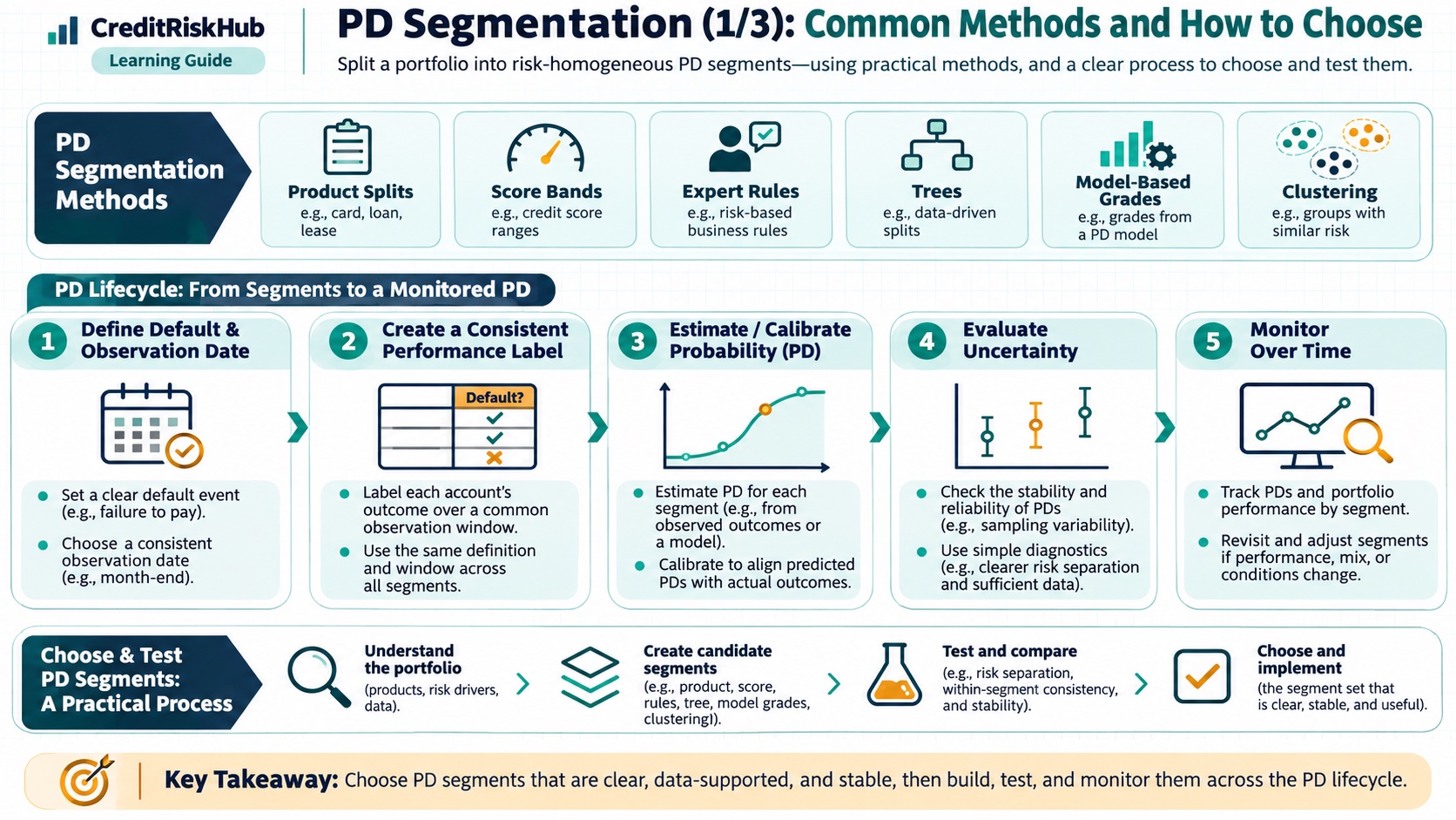
A useful segment should: separate risk in a way supported by matured outcomes; have interpretable drivers and assignment rules; remain sufficiently populated; be stable enough to operate; and lead to a decision or monitoring action. Increasing segment count almost always makes in-sample rates look more detailed, but can make estimates noisy and operationally fragile.

1. Product or portfolio rules

Separate products, borrower types, regions, origination channels, collateralProperty or another asset pledged to support repayment or recovery after borrower default.Open full glossary entry ↗, or underwriting regimes when their risk processes genuinely differ. This is transparent and often the right first cut. Test that the distinction is backed by outcomes rather than convention alone.

2. Score or rating bands

Rank accounts with an existing score, then create grades using fixed cutoffs, quantiles, or calibrated risk bands. Quantiles balance the number of observations but do not guarantee similar risk or stable future sizes. Choose and document cutoffs on development data, then freeze them for out-of-time evaluation.

3. Expert-defined rules

Subject matter experts can define segments where product mechanics or policy create known differences, such as delinquent versus current accounts or secured versus unsecured lending. Keep overrides explicit and review override frequency, rationale, and outcomes; do not bury judgment inside undocumented data transformations.

4. Statistical trees and recursive partitioning

A classification tree can find feature splits that separate default outcomes. It is easy to visualize, but deep trees can overfit rare defaults and create tiny leaves. Use pruning or depth/minimum-leaf constraints chosen inside development data, then evaluate on a later period. Tree leaves are not calibrated PDs automatically.

5. Model-based risk bands

Logistic regressionA generalized linear model that links predictors to the log-odds of a binary outcome and can produce probability estimates.Open full glossary entry ↗ or another supervised model can estimate a continuous score; bands can then group similar predicted risk or support operational decisions. CalibrationAgreement between predicted probabilities and observed event frequencies for a matched population and horizon.Open full glossary entry ↗ may still be required for the intended population and horizon. Validate ranking and probability accuracy separately.

6. Clustering

Unsupervised methods group accounts by feature similarity, not by default risk. Clusters can help explore portfolio structure or identify different business processes, but must be tested against default outcomes and interpreted. A cluster is not a risk grade merely because it has a name.

7. Separate models versus pooled models

Fit separate models when populations have materially different drivers and enough data. Otherwise, a pooled model with interactions, hierarchical shrinkage, or segment-level calibration may reduce variance while allowing measured differences. Compare methods on the same time-based holdout and account for added complexity.

Step 1 — Define the target and perimeter

Specify default definition, forecast horizon, exposure grain, eligibility, and treatment of restructures, missing outcomes, and repeated borrowers. Keep the definition fixed through development and testing.

Step 2 — Map plausible risk drivers

Start with features known at the prediction date: borrower characteristics, product/transaction terms, payment behaviour, collateral, vintage, and relevant macroeconomic context. Exclude post-outcome information and variables that would not be available at scoring time.

Step 3 — Create candidate groups

Start with business segments and score bands, then examine simple rules or constrained trees if there is evidence of remaining heterogeneity. Avoid using future outcomes to define the groups being evaluated.

Step 4 — Check sample support and risk ordering

For each candidate segment report obligorA borrower or counterparty whose credit quality or default risk is assessed.Open full glossary entry ↗ count, matured defaults, exposure, average forecast PD, observed default rate, and uncertainty interval. Check whether risk rises in the expected direction, and investigate exceptions rather than forcing monotonicity without justification.

Step 5 — Compare on time

Choose development, validation, and out-of-time windows that respect event maturity and the way the model will be used. Compare calibration, ranking, stability, coverage, explainability, and operational effort. If multiple records belong to one borrower, keep the borrower from leaking across splits.

Step 6 — Freeze assignment and governance

Version the rules, thresholds, model, data, and default definition. Document who owns changes, approvals, exception handling, monitoring frequency, and rollback procedures.

A lender begins with 12,000 matured one-year observations. A transparent product split gives 8,000 installment loans and 4,000 revolving accounts. On a time-separated validation sample, observed default rates are 2.1% and 5.8%, respectively, with adequate defaults in both groups. This suggests a product-level difference worth investigating; it does not prove that separate models are needed. Compare separate calibration on the same holdout with a pooled model that includes product and relevant interactions, and check stability over later vintages.

Every segmentation choice creates a future monitoring obligation. Preserve segment counts, exposure shares, grade migrations, missing or unassigned cases, score distributions, and matured observed-versus-expected outcomes. Track both portfolio-level and segment-level results: aggregate calibration can hide offsetting errors. Do not declare a group “bad” from a short window with few defaults; disclose uncertainty and outcome maturity.

Keep accounting ECL, regulatory capital, and internal risk measures distinct. IFRS 9 staging and lifetime expected credit loss use accounting requirements and reporting-date assumptions; Basel IRB segmentation and PD estimation have prudential requirements for their relevant scope; internal segmentation follows its stated decision use and governance. Reusing a model component does not make the resulting measures interchangeable.

No segmentation method can compensate for inaccurate labels, leakage, changing underwriting policy, poor linkage, or an unrepresentative sample. Risk similarity is relative to a target, horizon, period, and use. A group can be homogeneous on average but contain an important subgroup. Keep a sensible number of groups and report uncertainty instead of promising precisionAmong cases predicted positive at a threshold, the proportion that are truly positive under the defined label.Open full glossary entry ↗ that the data do not support.

Basel Framework, CRE 36 — IRB approach minimum requirements, including meaningful risk differentiation, homogeneous retail pools, rating-system design, and validation: https://www.bis.org/committees/bcbs/basel-framework/standard/cre/36/inforce/2023-01-01/published/2020-03-27

Educational guide. Example populations and rates are synthetic. Choose methods, estimates, and controls for the intended portfolio and applicable accounting or regulatory framework.