Probability of default (PD)
PD calibration: point-in-time and through-the-cycle
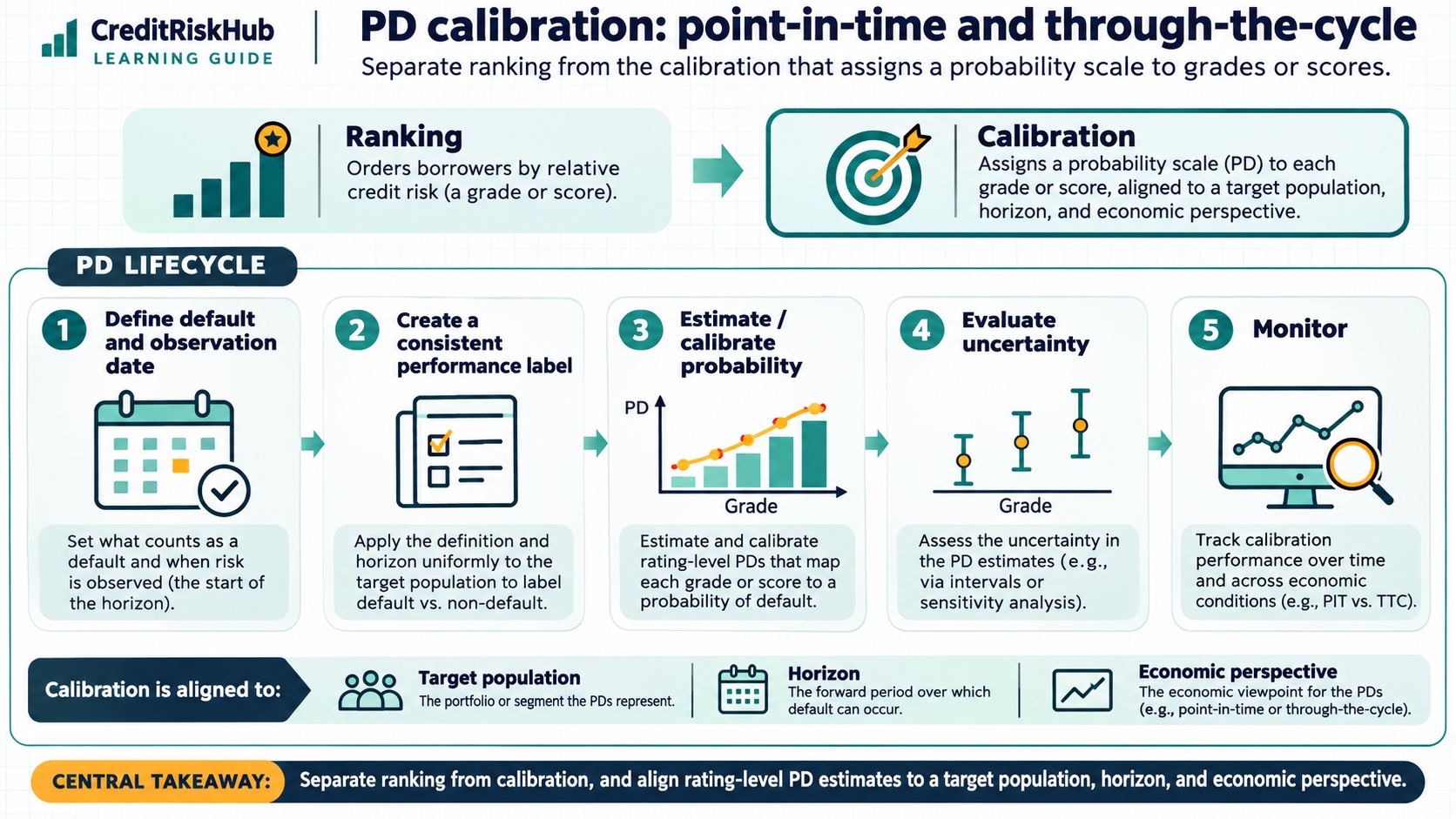
Separate ranking from the calibration that assigns a probability scale to grades or scores.
Purpose
Explain how rating-level PD estimates are aligned to a target population, horizon, and economic perspective.
Key terms
Hover over or focus a term for a quick definition, or open its glossary entry.
Key definitions
- Calibration maps a score or grade to a probability level.
- Point-in-time estimates reflect current conditions; through-the-cycle estimates seek a longer-run perspective, with definitions varying by institution and use.
Grade calibration example = defaults in grade over horizon ÷ eligible grade population.Worked example
A grade with 18 observed defaults among 1,200 fully observed obligors has a raw one-year rate of 1.5% before uncertainty or conditioning adjustments.
Detailed explanation
A score can rank borrowers well and still assign probabilities that are too high or too low. Calibration estimates the probability scale for a named population, horizon, and time perspective. A grade-level observed rate is a simple starting point, but should be checked for sample size, representativeness, default definition, and changes in the business or macro environment.
Point-in-time and through-the-cycle are approaches to conditioning and smoothing, not interchangeable labels for one fixed formula. Explain which data periods, macro adjustments, and long-run averaging rules are used. For IFRS 9, forward-looking information and reporting-date conditions matter; a prudential long-run calibration should not be reused without a purpose-specific bridge.
Try a reproducible Python example
These examples use synthetic inputs and run locally in a browser worker. Edit the code, run it, and compare its output with the published example.
Runnable Python · local in your browser
Convert a logistic model logit to PD
Apply the logistic function to an illustrative intercept plus two feature contributions.
Output
Run the code to see the output.
Runtime loads only after you press Run. Code runs in a separate browser worker with a 10-second limit and a 20,000-character output cap. Use synthetic examples only; browser execution is not a secure environment for secrets or sensitive records.
Runnable Python · local in your browser
Calculate year-by-year marginal and cumulative PD
Follow years 1–3 separately: conditional PD is the rate among survivors, marginal PD is the share of the original cohort defaulting in that year, and cumulative PD adds those marginal shares.
Output
Run the code to see the output.
Runtime loads only after you press Run. Code runs in a separate browser worker with a 10-second limit and a 20,000-character output cap. Use synthetic examples only; browser execution is not a secure environment for secrets or sensitive records.
Assumptions
- The calibration sample and target definition match the intended use or are adjusted transparently.
Limitations
- A raw rate can be noisy in small or low-default grades.
- PIT/TTC labels are not universal mathematical definitions; document the actual method.
References
- Basel Framework: IRB approach and credit-risk components — Basel Committee on Banking Supervision
- IFRS 9 Financial Instruments — IFRS Foundation
- Guidelines on PD estimation, LGD estimation and treatment of defaulted assets — European Banking Authority
Educational material only. Methods and examples are simplified; state and validate the assumptions required for your use case.