Probability of default (PD)
Estimating a One-Year Probability of Default
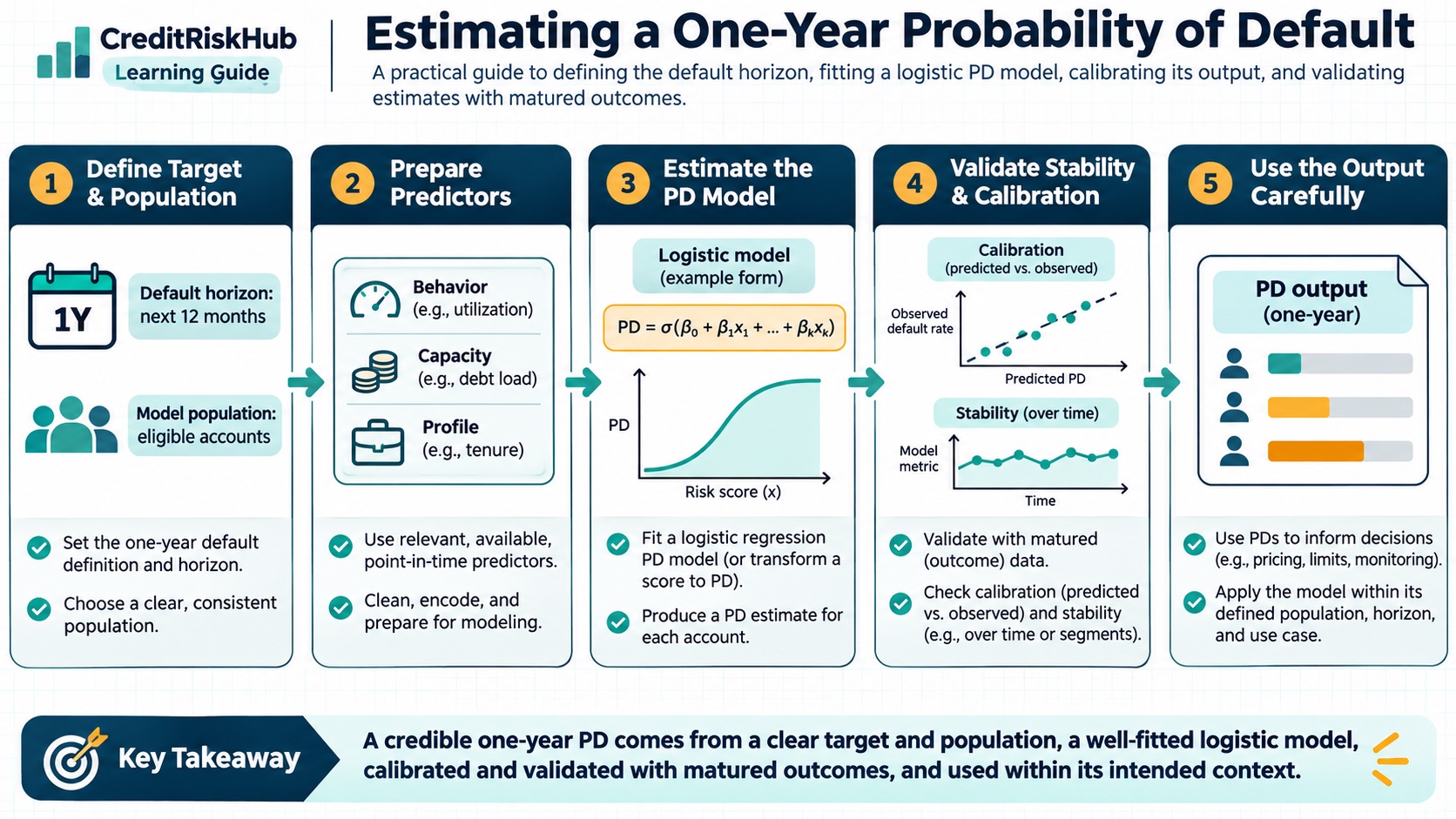
A practical guide to defining the default horizon, fitting a logistic PD model, calibrating its output, and validating estimates with matured outcomes.
Updated 2026-10-24
Purpose
A practical guide to defining the default horizon, fitting a logistic PD model, calibrating its output, and validating estimates with matured outcomes.
Key terms
Hover over or focus a term for a quick definition, or open its glossary entry.
Basel Framework, CRE 32 (IRB risk components, including PD): https://www.bis.org/basel_framework/chapter/CRE/32.htm?inforce=20230101&published=20200327
Basel Framework, CRE 36 (minimum requirements for IRB estimates): https://www.bis.org/basel_framework/chapter/CRE/36.htm?inforce=20230101&published=20200327
WHAT A ONE-YEAR PD MEASURES
A probability of default (PD) is the estimated chance that an obligor will meet a defined default event over a stated horizon, conditional on information available at the measurement date. A one-year PD refers to default during the next 12 months. It is meaningful only when the population, unit of analysis, default definition, observation date, and outcome horizon are specified. Basel’s IRB framework uses a one-year PD for corporate, sovereign, and bank exposures; a model score alone does not establish that a PD meets regulatory requirements.
Define default before building labels. The definition may include both days-past-due criteria and unlikeliness-to-pay events, subject to applicable policy and jurisdiction. Apply it consistently to development, validation, and monitoring data. Link related accounts to obligors where the target is obligor default, set the observation date before the outcome window, and exclude features that were not available on that date. These choices determine what the model learns.
BUILD A POINT-IN-TIME DEVELOPMENT SAMPLE
Create one observation per eligible obligor at a defined date, with predictor values reconstructed as they were known then. Mark the target as one when the defined default occurs within the following 12 months, and zero only when the full horizon is observed without default. Recent observations whose outcome windows have not matured are censored; treating them as non-defaults biases measured default rates downward. Document exclusions, restructures, cures, and repeat observations.
Split samples by time where possible: develop on earlier periods, tune on a later period, and reserve a fully out-of-time period for final validation. Keep all observations from the same obligor together when repeated records could otherwise leak across splits. Review missingness, outliers, category changes, and population coverage before fitting. A statistically strong model can still be unreliable if the historical data does not represent the intended use population.
ESTIMATE A LOGISTIC PD MODEL
A common scorecard approach estimates a linear predictor, or logit, from approved features: z = β₀ + β₁x₁ + … + βₖxₖ. Convert it to a probability with the logistic function: PD = 1 / (1 + exp(−z)). Coefficients describe conditional associations in the fitted sample; they are not causal effects. Feature transformations, binning, regularization, and variable selection should be justified, stable, and checked for leakage and unreasonable relationships.
For illustration only, suppose an intercept of −3.2 and two feature contributions of +0.35 and +1.10 produce a logit of −1.75. The logistic transform gives a raw PD of about 14.8%. Those values are synthetic and say nothing about a real borrower or portfolio. The guide page includes a matching browser-based Python cell that you can edit and run locally using synthetic values.
CALIBRATE THE ESTIMATE TO ITS TARGET POPULATION
Discrimination asks whether higher-risk obligors tend to rank above lower-risk obligors. Calibration asks whether predicted probabilities agree with realized frequencies over the stated horizon. Assess calibration on matured, representative observations using multiple views: observed versus predicted default rates by risk band, observed-to-expected totals, calibration plots, and suitable probability scores. Include confidence intervals or sample counts so unstable estimates in small segments are visible.
If a model ranks well but systematically overpredicts or underpredicts, investigate changes in the population, default definition, sample weighting, economic conditions, and development-to-application differences. Any recalibration should preserve the intended target and be documented, independently reviewed, and monitored. A single portfolio-level adjustment can conceal offsetting errors across segments, so inspect relevant product, vintage, geography, and risk bands where data supports them.
VALIDATE AND MONITOR OVER TIME
Use complementary measures rather than relying on one headline statistic. ROC-AUC or Gini can summarize ranking; Brier score and log loss assess probability accuracy; observed-to-expected and calibration plots reveal systematic bias. Track data quality, missingness, feature and score distributions, approval or selection effects, and the maturity of outcome windows. Define escalation limits using portfolio size, uncertainty, risk appetite, and intended use; there is no universal threshold that is appropriate for every portfolio.
Compare current performance with the development and validation baselines, investigate material shifts, and record remediation decisions. Monitor at a frequency suited to the product’s risk and data availability. A one-year outcome requires time to mature, so use interim indicators carefully and do not present them as completed one-year validation. Maintain versioned data definitions, code, coefficients, calibration steps, approvals, and limitations so results can be reproduced.
KEEP REGULATORY AND ACCOUNTING PURPOSES DISTINCT
A Basel IRB one-year PD and an IFRS 9 expected-credit-loss estimate answer different questions. IFRS 9’s 12-month ECL represents the lifetime cash shortfalls associated with default events that are possible in the 12 months after the reporting date, weighted by the probability of those defaults; it is not simply the cash shortfall expected to be paid during the next 12 months. IFRS 9 ECL measurement also requires probability-weighted, reasonable and supportable information, including relevant forward-looking conditions.
Do not treat a regulatory PD as an IFRS 9 provision input without assessing the target definition, measurement date, horizon, scenario conditioning, and the other ECL components. PD, loss given default, exposure at default, discounting, staging, and scenario weighting must be aligned to the applicable accounting policy. This guide is educational and does not replace institutional model governance, supervisory requirements, or accounting advice.
REFERENCES
IFRS 9 Financial Instruments, paragraphs B5.5.17 and B5.5.43: https://www.ifrs.org/content/dam/ifrs/publications/pdf-standards/english/2021/issued/part-a/ifrs-9-financial-instruments.pdf
Try a reproducible Python example
These examples use synthetic inputs and run locally in a browser worker. Edit the code, run it, and compare its output with the published example.
Runnable Python · local in your browser
Convert a logistic model logit to PD
Apply the logistic function to an illustrative intercept plus two feature contributions.
Output
Run the code to see the output.
Runtime loads only after you press Run. Code runs in a separate browser worker with a 10-second limit and a 20,000-character output cap. Use synthetic examples only; browser execution is not a secure environment for secrets or sensitive records.
Runnable Python · local in your browser
Calculate year-by-year marginal and cumulative PD
Follow years 1–3 separately: conditional PD is the rate among survivors, marginal PD is the share of the original cohort defaulting in that year, and cumulative PD adds those marginal shares.
Output
Run the code to see the output.
Runtime loads only after you press Run. Code runs in a separate browser worker with a 10-second limit and a 20,000-character output cap. Use synthetic examples only; browser execution is not a secure environment for secrets or sensitive records.
References
- Basel Framework; IFRS 9 — Basel Framework; IFRS 9
Educational material only. Methods and examples are simplified; state and validate the assumptions required for your use case.