Probability of default (PD)
Default Rate, Observation Window, and Performance Period: Choosing 60 or 90 DPD
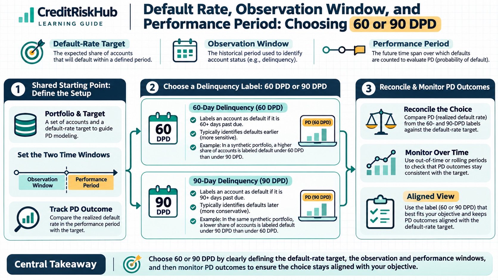
Define default-rate targets, distinguish observation and performance windows, compare 60- and 90-day delinquency labels, and monitor PD outcomes with synthetic examples.
Updated 2026-10-28
Purpose
Define default-rate targets, distinguish observation and performance windows, compare 60- and 90-day delinquency labels, and monitor PD outcomes with synthetic examples.
Key terms
Hover over or focus a term for a quick definition, or open its glossary entry.
Observed default rate over H = distinct eligible obligors with at least one qualifying default during (t0, t0 + H] ÷ eligible non-defaulted obligors at t0.A probability-of-default model is only as clear as its outcome label. “Default rate” can mean the rate of borrowers entering a defined default state over a stated horizon, while “60 days past due” and “90 days past due” are operational delinquency rules that may or may not equal the default definition used for a regulatory or accounting purpose. If the target, unit of analysis, dates, and treatment of incomplete observations are ambiguous, both the model and its monitoring metrics become hard to interpret.
This guide defines the key time windows, shows how to calculate an observed default rate, compares 60- and 90-day delinquency labels, and gives a practical validation workflow. The examples use synthetic data. The choice of label must fit the intended use and the governing policy; the examples do not set a universal default rule.
DEFINE DEFAULT BEFORE COUNTING IT
A default event is a labelled credit outcome, not merely any late payment. For Basel IRB, the reference definition identifies default when the bank considers the obligor unlikely to pay its credit obligations in full without actions such as realizing security, or when the obligor is more than 90 days past due on a material credit obligation. Basel includes other unlikeliness-to-pay indicators and allows supervisors to substitute a longer days-past-due period for specified retail or public-sector exposures under applicable rules. A days-past-due trigger is therefore one part of a broader prudential definition. See Basel Framework CRE36.69–36.76 (https://www.bis.org/basel_framework/chapter/CRE/36.htm?inforce=20230101&published=20221208).
For IFRS 9, an entity uses a default definition consistent with its internal credit-risk-management definition for the relevant instrument and considers qualitative indicators where appropriate. The Standard includes a rebuttable presumption that default does not occur later than 90 days past due unless reasonable and supportable information demonstrates that a more lagging criterion is more appropriate. A 30-day-past-due backstop is a separate IFRS 9 indicator for a significant increase in credit risk (SICR); it does not itself redefine default. See IFRS 9 paragraphs B5.5.17 and B5.5.37 in the IFRS Foundation’s issued Standard (https://www.ifrs.org/content/dam/ifrs/publications/pdf-standards/english/2021/issued/part-a/ifrs-9-financial-instruments.pdf?bypass=on).
Write the target as a complete rule. Specify whether it is obligor-level or facility-level, which obligations count, the materiality rule, the treatment of unlikeliness-to-pay events, how days past due are counted, when default begins and ends, and whether a later re-default is a new event for the model’s purpose. Do not count multiple accounts for one borrower as independent borrowers unless the model and validation are intentionally facility-level. For regulatory estimates, follow the local implementation of the relevant framework. For IFRS 9, keep the accounting default definition consistent with internal credit risk management and document any rebuttal of the 90-day presumption.
THREE DIFFERENT TIME WINDOWS
The feature lookback window is the period before a prediction date used to calculate predictors. For example, a model scored on 31 March might use payment behaviour from the previous six months. Every predictor must be available as of 31 March; later information must not leak into the score.
The historical observation period is the span of past data cohorts used to develop, calibrate, and validate the model. It might include several annual cohorts and multiple economic conditions. It is not the future horizon being predicted. For Basel IRB corporate, sovereign, and bank PD estimates, the Basel Framework requires at least five years of historical observation data for at least one source, with relevant longer data used; distinct requirements apply to retail exposures. That is a scoped prudential requirement, not a universal minimum for every business model or every internal score. See Basel Framework CRE36.78–36.83 (https://www.bis.org/basel_framework/chapter/CRE/36.htm?inforce=20230101&published=20221208).
The performance period is the future window after the observation date during which you look for the outcome. If the score estimates a one-year PD, an eligible non-defaulted borrower at time t0 is followed from t0 through t0 plus twelve months. If the intended measure is a lifetime PD, the horizon is the remaining expected life defined for that instrument and use. State the start and end dates and how an event on the boundary is handled.
CALCULATE A DEFAULT RATE FOR A STATED HORIZON
For a cohort of eligible non-defaulted obligors at time t0, a simple observed horizon default rate is:
For a one-year rate, H is twelve months. The numerator counts each obligor once for that one-year cohort even if the borrower has more than one default trigger or episode in the window. The denominator is established at the start of the period and must use the same unit of analysis. For example, a borrower-level numerator paired with an account-level denominator is invalid.
In the EU IRB context, EBA guidance specifies a one-year default-rate denominator of non-defaulted obligors with a credit obligation at the beginning of the period, and a numerator of those obligors that have at least one default during the period. Multiple defaults of the same obligor during that one-year observation period count as one in that period’s numerator. Apply the jurisdiction’s binding rules where relevant; a general product dashboard may have a different descriptive denominator if it labels the measure clearly. See EBA Guidelines on PD and LGD estimation, section 5.3.2 (https://www.eba.europa.eu/sites/default/files/documents/10180/2192133/f5a2e068-dc4b-4a0e-a10f-378b517ac19c/Guidelines%20on%20PD%20and%20LGD%20estimation%20%28EBA-GL-2017-16%29_EN.pdf).
SYNTHETIC ONE-YEAR EXAMPLE
At 31 March, a synthetic portfolio has 1,000 distinct active borrowers with no prior default. Each borrower has a complete twelve-month observation window ending the next 31 March. Thirty-five borrowers meet the specified default definition at least once during that window. The observed one-year default rate is 35 / 1,000 = 3.5%. If the same 35 borrowers generated 48 default records because of multiple facilities or repeated triggers, the borrower-level numerator remains 35 for this cohort.
Suppose 58 borrowers also reached 60 DPD during the same window. The 60-DPD event rate is 58 / 1,000 = 5.8%, provided 60 DPD is precisely defined and measured at the selected unit. It is a different outcome from the 3.5% default rate. These rates can overlap, but one does not automatically equal the other. Some borrowers may cure after 60 DPD; others may enter default through unlikeliness to pay before reaching a day-count threshold.
CHOOSING 60 DPD OR 90 DPD
There is no universally best delinquency threshold. Choose the event that matches the decision and name it accurately. A 90-DPD label may align more closely with a common regulatory backstop and produce a more severe, usually less frequent event. It is still not a complete default definition where unlikeliness-to-pay indicators can trigger default earlier. A 60-DPD label can provide an earlier collections or early-warning signal and may yield more examples, but it captures a broader group that may include borrowers who cure without meeting the formal default definition.
If the model is intended to estimate regulatory default PD or IFRS 9 default risk, do not replace the applicable default definition with 60 DPD simply because it improves class balance, model performance, or speed. Use 60 DPD as a separately named delinquency target only when that is the intended outcome, such as “probability of reaching 60 DPD within 12 months.” Do not call it default PD unless the governing definition actually makes that event default. Likewise, 30 DPD has an explicit role as an IFRS 9 SICR backstop in specified circumstances, but it is not itself the default threshold.
Compare candidate labels before adopting one. On a mature development cohort, report event counts, event rates, time from score date to event, cure rates after each DPD threshold, re-defaults, and event overlap. Review results by product, customer type, risk band, and vintage. Ask whether the outcome is observable early enough for the intended action, stable enough to estimate, and aligned with policy and downstream accounting or capital use. Have credit-risk, collections, finance, and regulatory owners approve the label where their uses depend on it.
CHOOSE THE PERFORMANCE PERIOD FROM THE USE CASE
A one-year performance period is a common target when the output is a one-year PD. It also aligns with Basel IRB’s one-year PD concept for the relevant regulatory grades and pools. It does not mean every credit decision should use a twelve-month outcome. A collections model may predict 60-DPD within three months; a renewal decision may need risk through a shorter contractual window; a lifetime PD curve needs multiple future periods. The label should say both the event and the horizon.
Longer horizons give more time for defaults to occur, so the cumulative event rate generally rises, but prediction uncertainty also grows. More accounts may prepay, close, refinance, or be lost to follow-up before the horizon ends. For a one-year target, only call an account non-default when the full year is observed and the account’s outcome is known under the chosen policy. Mark immature or unobserved outcomes as censored or not yet mature; do not silently classify them as good. For longer horizons, use survival methods or appropriately defined period-by-period targets when censoring and event timing matter.
Do not choose a performance period after repeatedly trying horizons until a preferred AUC or event rate appears. Define it from the decision, contract, and default-risk concept first; then test whether the available data can support that horizon. If you change the horizon, you change the target PD and should re-estimate and revalidate the model.
BUILD THE LABEL DATASET STEP BY STEP
1. Choose the unit: obligor, facility, account, or another governed entity
Keep it consistent in features, defaults, and denominators. 2. Define t0 and the eligibility rules. Exclude already-defaulted units from a non-default PD target, but keep a separate list to reconcile coverage. 3. Freeze the feature snapshot at t0. Store the feature timestamp and source so the model can be reconstructed without future information. 4. Create the target rule, including DPD calculation, materiality, qualitative default triggers, and date-boundary convention. 5. Observe the full performance period. Link all default events and closure events to the starting unit, accounting for migrations and multiple facilities under the chosen policy. 6. Assign labels: 1 if a qualifying event occurs in the performance window; 0 only if the full window is observed and no qualifying event occurs; censored/not mature if the outcome cannot yet be established. 7. Preserve an audit trail: source event IDs, event date, rule version, exclusions, cures, re-defaults, and any manual adjudication.
Split training and validation by time. If borrower-level observations repeat over several dates, keep the same borrower from leaking into both sides of a validation split where that would inflate performance. Build a final out-of-time cohort with fully mature outcomes. Check label counts and event rates against source systems before fitting a model.
VALIDATE AND MONITOR THE TARGET
Start with data and label quality: missing or duplicate IDs, default events without dates, DPD spikes, changing materiality or cure rules, incomplete performance windows, account closures, overrides, and unexplained movements in the share of censored cases. Reconcile the event count with the servicing or default-management system and sample records manually.
Monitor the observed default rate by cohort, product, grade or score band, customer type, and calendar period. Compare it with the average predicted PD for the same mature population. A simple observed-to-expected ratio is O/E = observed defaults / sum of predicted PDs. O/E near 1 indicates aggregate alignment for that sample; it does not prove correct ranking, stable calibration, or adequate sample size. Report default counts and confidence intervals alongside rates, especially for low-default portfolios.
Assess discrimination and calibration separately. AUC or Gini describes ranking, not whether the PD level is right. Calibration plots compare average predicted PD with observed default frequency by band. Calibration intercept and slope can reveal systematic level or spread errors when sample size supports them. Brier score measures squared probability error. Also track score and feature drift, population mix, transition rates between risk bands, and the time between observation and event. When a 60-DPD target is used, monitor cure after 60 DPD and the fraction later meeting the default definition; when a 90-DPD target is used, monitor unlikeliness-to-pay events that occur before 90 DPD.
Set review thresholds in advance and account for uncertainty. A small number of defaults can make rates move sharply from one period to the next. Investigate changing underwriting, collections, product limits, data capture, macro conditions, and policy definitions before recalibrating. Keep the target definition versioned so a change to 60/90 DPD or default criteria does not masquerade as model drift.
KEEP ACCOUNTING, REGULATORY, AND INTERNAL MEASURES SEPARATE
An IFRS 9 ECL estimate is a probability-weighted present value of cash shortfalls using reasonable and supportable historical, current, and forward-looking information. Its 12-month versus lifetime horizon is determined by the Standard’s impairment requirements and SICR assessment; it is not interchangeable with a 60-DPD business target. IFRS 9 does not support replacing judgment with a single mechanistic trigger for all circumstances. See the IFRS Foundation’s application material on IFRS 9 ECL (https://www.ifrs.org/news-and-events/news/2020/03/application-of-ifrs-9-in-the-light-of-the-coronavirus-uncertainty/).
A Basel IRB PD estimate must use the applicable default reference definition and regulatory quantification requirements, including a long-run average of one-year default rates for the relevant grades or pools. The precise requirements and any permitted local exceptions depend on exposure class and jurisdiction. An internal early-warning or collections model can use a 30-, 60-, or 90-DPD outcome if the business decision calls for it; label that outcome and horizon explicitly and do not present it as accounting ECL or regulatory PD without the required reconciliation and approval.
ASSUMPTIONS AND LIMITATIONS
• The counts and rates in the examples are synthetic. • “60 DPD” and “90 DPD” require a precise rule for due amounts, materiality, payment allocation, extensions, and the date on which the clock starts. • One-year default-rate calculations vary by regulatory framework and unit of analysis; the formula here is a general teaching representation, not a substitute for jurisdiction-specific requirements. • A simple default rate is not automatically a calibrated PD. It may need long-run, cohort, segmentation, and forward-looking adjustments for its intended use. • This guide is educational. Have qualified accounting, model-risk, and regulatory specialists approve definitions used in formal reporting or capital measurement.
REFERENCES
• Basel Committee on Banking Supervision, Basel Framework CRE36: IRB minimum requirements (https://www.bis.org/basel_framework/chapter/CRE/36.htm?inforce=20230101&published=20221208), including default definition, PD estimation, and historical observation-period requirements. • European Banking Authority, Guidelines on PD estimation, LGD estimation and treatment of defaulted exposures (https://www.eba.europa.eu/sites/default/files/documents/10180/2192133/f5a2e068-dc4b-4a0e-a10f-378b517ac19c/Guidelines%20on%20PD%20and%20LGD%20estimation%20%28EBA-GL-2017-16%29_EN.pdf), section 5.3.2 for one-year default-rate denominators and numerators. • IFRS Foundation, IFRS 9 Financial Instruments (https://www.ifrs.org/content/dam/ifrs/publications/pdf-standards/english/2021/issued/part-a/ifrs-9-financial-instruments.pdf?bypass=on), including paragraphs B5.5.17, B5.5.37, and the 30-days-past-due SICR presumption in B5.5.19. • IFRS Foundation, Application of IFRS 9 in the light of coronavirus uncertainty (https://www.ifrs.org/news-and-events/news/2020/03/application-of-ifrs-9-in-the-light-of-the-coronavirus-uncertainty/), emphasizing reasonable and supportable information and avoiding a mechanistic SICR approach.
Educational material only. Confirm the current accounting standard, prudential rules, and internal policy before applying a default label or PD estimate.
Try a reproducible Python example
These examples use synthetic inputs and run locally in a browser worker. Edit the code, run it, and compare its output with the published example.
Runnable Python · local in your browser
Convert a logistic model logit to PD
Apply the logistic function to an illustrative intercept plus two feature contributions.
Output
Run the code to see the output.
Runtime loads only after you press Run. Code runs in a separate browser worker with a 10-second limit and a 20,000-character output cap. Use synthetic examples only; browser execution is not a secure environment for secrets or sensitive records.
Runnable Python · local in your browser
Calculate year-by-year marginal and cumulative PD
Follow years 1–3 separately: conditional PD is the rate among survivors, marginal PD is the share of the original cohort defaulting in that year, and cumulative PD adds those marginal shares.
Output
Run the code to see the output.
Runtime loads only after you press Run. Code runs in a separate browser worker with a 10-second limit and a 20,000-character output cap. Use synthetic examples only; browser execution is not a secure environment for secrets or sensitive records.
References
- CreditRiskHub — CreditRiskHub
Educational material only. Methods and examples are simplified; state and validate the assumptions required for your use case.