IFRS 9 expected credit loss
IFRS 9 ECL Staging: A Step-by-Step Guide to 12-Month and Lifetime ECL
Understand IFRS 9’s three-stage general approach, assess significant increases in credit risk, and calculate 12-month versus lifetime ECL with a synthetic term-structure example.
Updated 2026-10-29
Purpose
Understand IFRS 9’s three-stage general approach, assess significant increases in credit risk, and calculate 12-month versus lifetime ECL with a synthetic term-structure example.
Key terms
Hover over or focus a term for a quick definition, or open its glossary entry.
mPDₜ = Sₜ₋₁ × hₜ
Sₜ₋₁ = Πᵢ₌₁ₜ₋₁ (1 − hᵢ)
Discounted ELₜ = mPDₜ × EADₜ × LGDₜ / (1 + EIR)ᵗ
Year 1: Survival at start is 100%. Marginal PD is 1.0000 × 2% = 2.0000%. Approximate discounted expected loss is 2.0000% × $100,000 × 35% / 1.08 = $648.15.
Year 2: Survival at start is 1 − 2% = 98%. Marginal PD is 98% × 3% = 2.9400%. Discounted expected loss is 2.9400% × $100,000 × 35% / 1.08² = $882.20.
Year 3: Survival at start is 98% × 97% = 95.06%. Marginal PD is 95.06% × 4% = 3.8024%. Discounted expected loss is 3.8024% × $100,000 × 35% / 1.08³ = $1,056.46.
The cumulative default probability through year 3 is 2.0000% + 2.9400% + 3.8024% = 8.7424%. The simplified lifetime ECL is approximately $648.15 + $882.20 + $1,056.46 = $2,586.81.
ECL = Σₛ wₛ × ECLₛ, with Σₛ wₛ = 1
PURPOSE AND SCOPE
IFRS 9’s expected credit loss (ECL) model changes the allowance measurement as credit risk changes after initial recognition. Under the general approach, the key decision is whether credit risk has increased significantly since the instrument was first recognised. That assessment determines whether the allowance is 12-month ECL or lifetime ECL; it is not a direct comparison of this period’s allowance with last period’s allowance.
This guide explains the general staging approach for a synthetic amortising loan. IFRS 9 also contains simplified approaches for specified receivables and contract assets, as well as instrument-specific requirements and exceptions. An implementation must follow the applicable accounting policy, instrument scope, jurisdictional adoption, and institution-approved interpretation.
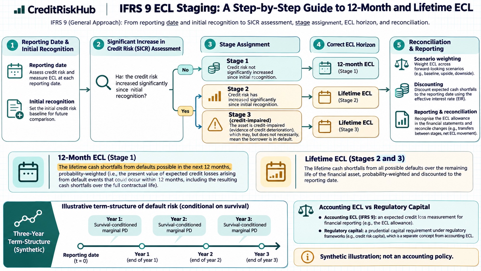
THE MODEL IN ONE PICTURE
The graphic below connects the staging decision to the measurement horizon. Its numbers use the same synthetic loan developed in the worked example.
THE THREE STAGES AT A GLANCE
Stage 1 — no significant increase in credit risk (SICR) since initial recognition: Measure the loss allowance at 12-month ECL. Continue to reassess at every reporting date.
Stage 2 — SICR since initial recognition, but the asset is not credit-impaired: Measure lifetime ECL. SICR is a change in the risk of default over the instrument’s expected life, assessed relative to risk at initial recognition and using reasonable and supportable information, including forward-looking information.
Stage 3 — credit-impaired at the reporting date: Measure lifetime ECL. Credit-impaired status is an accounting assessment under IFRS 9; it is not merely a particular internal rating label. Interest revenue has separate requirements for credit-impaired assets and is outside this numerical example.
A loan can move from Stage 2 back to Stage 1 if the SICR criteria are no longer met, based on the reporting-date assessment and policy. Staging is reassessed at each reporting date.
WHAT 12-MONTH ECL ACTUALLY MEANS
12-month ECL is the probability-weighted portion of lifetime cash shortfalls that would result if a default occurs in the next 12 months. It is not the sum of cash shortfalls expected to be paid during the next 12 months. A default during the next year can cause losses—such as delayed or missing repayments—that occur after that year; those consequences belong in the estimate for that default event.
Lifetime ECL considers the risk of default throughout the instrument’s expected life. In either measure, the objective is an unbiased, probability-weighted amount that reflects the time value of money and reasonable and supportable information available at the reporting date about past events, current conditions, and forecasts.
STEP 1: ESTABLISH THE ORIGINATION COMPARISON
At initial recognition, preserve a credible baseline for credit risk. Depending on the portfolio, this may include the borrower or facility’s initial lifetime default-risk estimate, rating or score, product and term, origination date, and relevant qualitative risk indicators. Store enough information to recreate the comparison at later reporting dates.
Do not use only the current risk level. SICR is assessed as a change since initial recognition. A given absolute increase can be more significant for a loan that began with very low default risk than for one that began with higher risk. Compare like with like: keep the default definition, horizon, segmentation, and model basis sufficiently consistent, and document any approved adjustments.
STEP 2: ASSESS SICR WITH QUANTITATIVE AND QUALITATIVE EVIDENCE
A practical process can include:
1. Estimate or otherwise assess the risk of default over the expected life at initial recognition and at the reporting date
2. Compare the change with documented, portfolio-appropriate SICR criteria
3. Add qualitative indicators and reasonable, supportable forward-looking information
A model score is evidence, not a substitute for judgment.
4. Apply the more-than-30-days-past-due rebuttable presumption as a backstop where relevant; any rebuttal needs support
Do not treat 30 days past due as the only SICR trigger or as the default definition.
5. Assess relevant exposures collectively when shared risk changes may not yet be visible at the individual-account level
6. Record the result, evidence, overrides, and approval trail
IFRS 9 does not prescribe one universal PD threshold for SICR. A threshold should be calibrated and governed for the product and portfolio, tested for timely identification, and supplemented where model inputs lag emerging risk. Low-credit-risk provisions are an operational simplification with conditions; an external investment-grade label alone should not automatically decide the assessment.
STEP 3: CALCULATE MARGINAL DEFAULT PROBABILITIES
For a term-structure example, let hₜ be the conditional probability of default in year t, given survival to the start of that year. The unconditional marginal probability of default in year t is:
where survival to the start of year t is:
The cumulative probability of default through year T is 1 − Sₜ, or equivalently the sum of marginal PDs through year T. Use probabilities on a consistent basis: do not add conditional hazards as if they were marginal probabilities.
WORKED SYNTHETIC EXAMPLE: STAGE 1 VERSUS STAGE 2
Assume a three-year loan has a constant exposure at default of $100,000, an illustrative loss given default of 35%, and an original effective interest rate of 8%. Assume defaults and their cash shortfalls are represented at each year-end. The conditional annual default probabilities are 2% in year 1, 3% in year 2 given survival to year 2, and 4% in year 3 given survival to year 3. These numbers are synthetic and are not a policy recommendation.
For this teaching example, estimate each period’s discounted expected loss as:
The same calculation in a compact table:
| Year | Conditional PD | Survival at start | Marginal PD | Discounted expected loss | | --- | ---: | ---: | ---: | ---: | | 1 | 2.00% | 100.00% | 2.0000% | $648.15 | | 2 | 3.00% | 98.00% | 2.9400% | $882.20 | | 3 | 4.00% | 95.06% | 3.8024% | $1,056.46 | | Lifetime total | — | — | 8.7424% cumulative PD | $2,586.81 |
The table summarizes the numerical example; retain the period-by-period steps above when reviewing the derivation.
If the loan is in Stage 1, the simplified 12-month ECL includes the year-1 default event and its full modeled loss consequences: approximately $648.15. It does not include year-2 and year-3 default events. If it is in Stage 2 or Stage 3, this illustration uses all three years, giving lifetime ECL of approximately $2,586.81.
This calculation is an educational PD × LGD × EAD approximation. Real IFRS 9 measurement may need to model contractual cash flows, expected prepayments, amortising or changing EAD, recovery timing, collateral and qualifying credit enhancements, scenario-dependent PD/LGD/EAD, and the correct effective-interest-rate discounting. The expected credit loss is defined by contractual cash shortfalls; PD × LGD × EAD is a modeling representation whose assumptions must match that objective.
STEP 4: PROBABILITY-WEIGHT SCENARIOS
Where economic scenarios change the estimated cash shortfalls, calculate an ECL for each coherent scenario and probability-weight them:
For example, a base scenario and a downside scenario should have internally consistent macro assumptions, default paths, exposure behavior, and recovery expectations. A management overlay should address a defined gap or limitation, avoid double counting risks already in the model, have an owner and evidence, and be monitored for release or recalibration. A simple average of optimistic and pessimistic outcomes is not automatically unbiased.
STEP 5: DISCOUNT CONSISTENTLY
Expected credit losses are measured at the reporting date. For most financial assets, IFRS 9 specifies discounting using the effective interest rate determined at initial recognition or an approximation; variable-rate instruments use the current effective interest rate determined under the Standard. There are specific rates for some instrument types, including purchased or originated credit-impaired assets and lease receivables. Confirm the relevant paragraph for the instrument before implementing the discounting rule.
The year-end discounting in the example is simplified. A production model should align expected shortfall timing with the contractual and expected cash-flow schedule rather than apply a generic year bucket when timing materially matters.
MONITORING AND CONTROLS
At each reporting date, monitor both the staging decision and the allowance measurement:
• Stage migration: balances and account counts moving between stages, by product, origination vintage, rating band, and risk segment. • SICR trigger performance: how early the policy and indicators flag accounts that later become delinquent, default, or credit-impaired; inspect overrides and rebuttals. • Origination baseline integrity: missing or overwritten origination risk, changes in score scales, inconsistent horizons, and backfilled data. • PD and loss calibration: compare predicted and observed outcomes using aligned default definitions and observation windows; account for censoring and low default counts. • ECL movement bridge: explain changes due to portfolio size, stage migration, risk parameters, macro scenarios, model changes, overlays, write-offs, and discount unwind. • Scenario governance: scenario weights, forecast horizon, reversion assumptions, sensitivity, and approval evidence. • Data and implementation controls: reconciliation to source balances, cash-flow completeness, duplicate or missing accounts, parameter versioning, and independent review of material model changes.
One metric cannot validate staging. For instance, stable total ECL can hide offsetting deterioration in risk and improvement in exposure or recoveries. Read portfolio totals alongside migrations, segment results, and driver analysis.
KEEP ACCOUNTING ECL, REGULATORY CAPITAL, AND INTERNAL RISK MEASURES SEPARATE
IFRS 9 ECL is an accounting allowance measured under the applicable reporting standard. Regulatory capital expected loss and capital requirements are determined by prudential rules, which can use different horizons, parameter definitions, and adjustments. Internal risk measures support decisions such as pricing, limits, and portfolio steering. Shared data and models can be useful, but outputs are not interchangeable without documented transformation, reconciliation, and governance.
COMMON ERRORS TO AVOID
• Treating 12-month ECL as only cash shortfalls paid in the next 12 months. • Using a 12-month PD as the sole SICR test for every instrument and portfolio. • Confusing a 30-DPD SICR backstop with the institution’s default definition. • Comparing current lifetime risk to a generic portfolio average rather than the instrument’s origination risk. • Adding conditional annual PDs without converting them to marginal PDs. • Applying one flat LGD, EAD, or discount factor across periods when expected cash shortfalls materially vary. • Treating a regulatory expected-loss output as IFRS 9 ECL without reconciling its purpose and assumptions. • Allowing overlays or overrides to persist without evidence, ownership, and monitoring.
REFERENCES
• IFRS Foundation, IFRS 9 Financial Instruments (https://www.ifrs.org/issued-standards/list-of-standards/ifrs-9-financial-instruments/), including paragraphs 5.5.3–5.5.5 and 5.5.17 and application guidance B5.5.7, B5.5.17, B5.5.43–B5.5.48. The standard defines the staging, measurement, probability-weighting, information, and discounting requirements. • IFRS Foundation, IFRS 9 and COVID-19: accounting for expected credit losses (https://www.ifrs.org/content/dam/ifrs/supporting-implementation/ifrs-9/ifrs-9-ecl-and-coronavirus.pdf?la=en), educational material reiterating SICR and use of reasonable and supportable forward-looking information; it does not amend the Standard. • Basel Committee on Banking Supervision, Guidance on credit risk and accounting for expected credit losses (https://www.bis.org/publications/201512-guidelines-guidance-credit-risk-and-accounting-expected-credit-losses), supervisory guidance for accounting ECL practices; it explicitly does not set regulatory capital expected-loss requirements.
Educational material using synthetic values only. It is not accounting, audit, or regulatory advice. Apply the current adopted Standard and institution-approved policy to the actual instrument and jurisdiction.
Try a reproducible Python example
These examples use synthetic inputs and run locally in a browser worker. Edit the code, run it, and compare its output with the published example.
Runnable Python · local in your browser
Calculate year-by-year marginal and cumulative PD
Follow years 1–3 separately: conditional PD is the rate among survivors, marginal PD is the share of the original cohort defaulting in that year, and cumulative PD adds those marginal shares.
Output
Run the code to see the output.
Runtime loads only after you press Run. Code runs in a separate browser worker with a 10-second limit and a 20,000-character output cap. Use synthetic examples only; browser execution is not a secure environment for secrets or sensitive records.
Runnable Python · local in your browser
Calculate survival-weighted, discounted ECL
Combine period marginal PD, LGD, EAD, discount factors, and two scenario weights in a small illustrative horizon.
Output
Run the code to see the output.
Runtime loads only after you press Run. Code runs in a separate browser worker with a 10-second limit and a 20,000-character output cap. Use synthetic examples only; browser execution is not a secure environment for secrets or sensitive records.
References
- IFRS Foundation; Basel Committee on Banking Supervision — IFRS Foundation; Basel Committee on Banking Supervision
Educational material only. Methods and examples are simplified; state and validate the assumptions required for your use case.