Exposure at default (EAD)
Lifetime EAD Backtesting: Methods, Metrics, and a Python Example
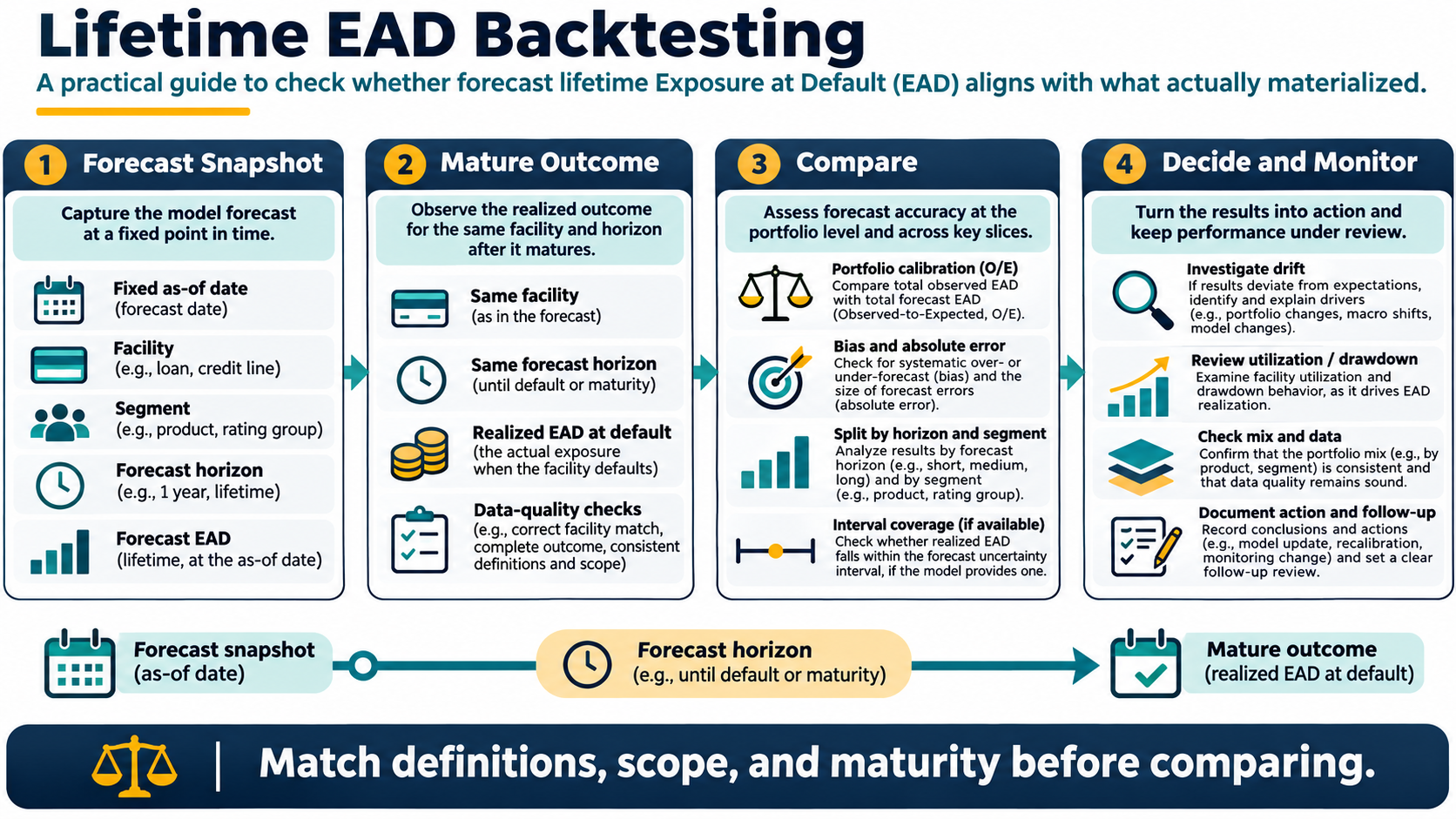
A practical guide to backtesting lifetime exposure-at-default forecasts: define mature cohorts, compare horizon-specific exposure, monitor calibration and error, and run deterministic Python with synthetic data.
Updated 2026-11-04
Purpose
A practical guide to backtesting lifetime exposure-at-default forecasts: define mature cohorts, compare horizon-specific exposure, monitor calibration and error, and run deterministic Python with synthetic data.
Key terms
Hover over or focus a term for a quick definition, or open its glossary entry.
O/E = Σ realized EAD ÷ Σ forecast EAD
Mean error = mean(forecast EAD − realized EAD)
MAE = mean(|forecast EAD − realized EAD|)
WAPE = Σ |forecast EAD − realized EAD| ÷ Σ realized EAD
Coverage = count(lower ≤ realized EAD ≤ upper) ÷ count(eligible outcomes)
Expected overall output: O/E = 1.043, mean error = −$650, MAE = $1,650, WAPE = 10.38%, interval coverage = 75.0%. Values in the input are thousands of dollars, so the code multiplies dollar error statistics by 1,000 for display.
Detailed explanation
Lifetime EAD Backtesting: Methods, Metrics, and a Python Example
Summary. A useful lifetime exposure-at-default backtest compares forecasts frozen at a known reporting date with outcomes observed later, using the same facilities, exposure definition, horizons, and eligibility rules. It reports portfolio calibration and error, then drills into time, horizon, and product segments. This guide uses synthetic values only.
1. What is being backtested?
Exposure at default (EAD) is the exposure amount associated with a defined default event. A lifetime EAD forecast is a path or set of horizon-specific estimates from an observation date through the expected life of a facility. It can support internal exposure planning and, as one input, expected-credit-loss models. It is not automatically the same thing as an IRB regulatory EAD estimate.
The target must say what counts as exposure: drawn principal, accrued interest, fees, commitments, limit excesses, currency conversion, and whether the measure is a point-in-time balance or a discounted cash-flow input. Forecast and realized values must follow the same approved definition. For committed and revolving products, distinguish forecast utilization or drawdown from exposure conditional on a default occurring.
A backtest answers: “For the defined population and maturity rule, how close were the archived forecasts to the realized outcomes?” It does not answer whether the model is suitable for every decision or regulatory purpose.
2. Three purposes that must stay distinct
PurposeWhat is being assessedKey distinction
Internal risk forecasting
Exposure paths for limits, stress analysis, planning, or pricing
Match the target and horizon to the intended decision.
Basel IRB parameter validation
The prescribed regulatory EAD parameter and its reference data
Basel CRE36 specifies a 12-month fixed-horizon setup for EAD estimation and requires robust validation; confirm the applicable local implementation and permission.
IFRS 9 accounting
Probability-weighted present value of contractual cash shortfalls
Expected drawdowns on loan commitments over the relevant 12-month or lifetime horizon matter. EAD is a modeling component; an EAD-only backtest does not validate ECL measurement.
3. Design the test before measuring performance
Freeze forecasts. Store one immutable row for each facility, observation date, horizon, and model version. Include the input snapshot, segment, forecast EAD, currency, and any forecast interval. Do not rebuild historical forecasts with information learned later.
Define the unit and default event. Decide whether the row is at obligor, facility, or account level, and whether first default, re-default, or default episode is being tested. Apply the same default policy throughout.
Choose horizon points. For example, test 12, 24, and 36 months, plus contractual or expected maturity where appropriate. Compare each horizon separately before showing an aggregate. A single pooled number can hide horizon drift.
Set outcome maturity. Include only rows whose full horizon has elapsed or whose default outcome can be observed under an explicitly defined early-default rule. Exclude or separately identify censored accounts, open facilities, missing outcomes, and prepayments. Never treat “not observed yet” as “no error.”
Reconcile exposure. Align the forecast and actual on facility identifier, default date, valuation date, currency and FX rate, inclusions, limit treatment, and exposure cut-off. Record changes in policy or servicing that could alter utilization.
Keep an untouched validation period. Use development data for model building and a later out-of-time sample for performance. For overlapping lifetime horizons, account for repeated facilities or observation windows in uncertainty estimates; naive row-level confidence intervals can be too narrow.
Report counts and coverage. Show number of eligible forecasts, mature outcomes, defaults, exclusions, censored rows, and total exposure. A metric without denominators is hard to interpret.
4. Useful comparison methods
A. Portfolio calibration: observed divided by expected
For matched records, calculate the sum of realized exposure divided by the sum of forecast exposure. A value above 1 indicates aggregate under-forecasting; below 1 indicates aggregate over-forecasting. This is exposure-weighted and can be dominated by a few large facilities, so show the distribution and segment results too.
B. Signed and absolute error
Mean signed error shows direction and can cancel large positive and negative errors. Mean absolute error (MAE) describes the average dollar miss. Weighted absolute percentage error (WAPE) scales total absolute error by total realized exposure. State the denominator and handle zero actual totals explicitly.
C. Segment and horizon analysis
Repeat calibration and error measures by forecast horizon, product, commitment type, utilization band, rating, vintage, geography, and size when sample support permits. Use pre-defined segment cuts; avoid creating slices after seeing outcomes solely to find favorable results. Include sample size, total exposure, and uncertainty for every material segment.
For facility-level error distribution, show median and upper-tail absolute errors in addition to averages. An overall O/E near one can coexist with offsetting over- and under-forecasting across products.
D. Prediction interval coverage
If the model provides lower and upper predictive bounds, calculate the share of realized outcomes inside the interval and show interval width. Coverage must be compared with the nominal level and assessed with enough observations; do not present a narrow interval as useful just because its coverage is high after the fact.
E. Time stability and operational checks
Plot O/E and error measures by forecast vintage and outcome month. Investigate movements in credit policy, line management, utilization, economic conditions, collections, default definitions, source-system logic, and portfolio mix. Monitor missingness, duplicate facility keys, stale snapshots, impossible negative balances, currency mismatches, and actual exposure above approved limits where those controls apply.
Use bootstrap intervals or another method that respects dependence (for example, resample obligors or facilities as clusters). The uncertainty method should match the sample design. Small samples are noisy; set thresholds from materiality, intended use, and empirical uncertainty, not a universal internet cutoff.
5. Worked synthetic example
The following eight matured default outcomes are synthetic and expressed in $000. Forecast intervals are illustrative only. Each record has a horizon and product segment, which makes it possible to see whether aggregate performance masks differences.
HorizonSegmentForecast EAD ($000)Realized EAD ($000)Illustrative interval ($000)Covered?
Year 1
Revolver
12.0
13.2
10.5–14.0
Yes
Year 1
Revolver
8.0
7.5
6.5–9.5
Yes
Year 1
Term
20.0
19.0
18.0–22.0
Yes
Year 1
Term
24.0
28.0
22.0–27.0
No
Year 2
Revolver
14.0
18.0
12.0–17.0
No
Year 2
Term
15.0
14.0
13.0–17.0
Yes
Year 2
Revolver
11.0
10.0
9.0–13.0
Yes
Year 2
Term
18.0
17.5
16.0–20.0
Yes
Across the eight outcomes, forecast exposure sums to $122,000 and realized exposure to $127,200. Observed-to-expected is 1.043: the forecast total is about 4.3% below the realized total. Mean forecast-minus-realized error is −$650 per record, MAE is $1,650, and WAPE is 10.38%. Six of eight realized values fall inside the illustrative intervals (75%). That interval result is not evidence of calibrated predictive uncertainty: eight records are far too few, and the intervals were chosen only for this example.
The horizon split is also informative: Year 1 O/E is 1.058 and Year 2 O/E is 1.026. Revolver O/E is 1.082, while term-loan O/E is 1.019. With these tiny counts, these splits are diagnostic prompts, not reliable conclusions. A production review would show many more mature facilities, confidence ranges, exposure concentration, and a pre-agreed materiality framework.
6. Runnable Python example
This code uses eight synthetic records, Python built-ins only, no external packages, no file, network, shell, or system calls. It calculates portfolio, horizon, segment, error, and interval summaries. It is deliberately small for browser execution.
rows = [ {"horizon": "Year 1", "segment": "Revolver", "forecast": 12.0, "actual": 13.2, "lower": 10.5, "upper": 14.0}, {"horizon": "Year 1", "segment": "Revolver", "forecast": 8.0, "actual": 7.5, "lower": 6.5, "upper": 9.5}, {"horizon": "Year 1", "segment": "Term", "forecast": 20.0, "actual": 19.0, "lower": 18.0, "upper": 22.0}, {"horizon": "Year 1", "segment": "Term", "forecast": 24.0, "actual": 28.0, "lower": 22.0, "upper": 27.0}, {"horizon": "Year 2", "segment": "Revolver", "forecast": 14.0, "actual": 18.0, "lower": 12.0, "upper": 17.0}, {"horizon": "Year 2", "segment": "Term", "forecast": 15.0, "actual": 14.0, "lower": 13.0, "upper": 17.0}, {"horizon": "Year 2", "segment": "Revolver", "forecast": 11.0, "actual": 10.0, "lower": 9.0, "upper": 13.0}, {"horizon": "Year 2", "segment": "Term", "forecast": 18.0, "actual": 17.5, "lower": 16.0, "upper": 20.0},]def summarize(group): predicted = sum(row["forecast"] for row in group) realized = sum(row["actual"] for row in group) errors = [row["forecast"] - row["actual"] for row in group] absolute_error = sum(abs(error) for error in errors) oe = realized / predicted if predicted else float("nan") wape = absolute_error / realized if realized else float("nan") coverage = sum(row["lower"] <= row["actual"] <= row["upper"] for row in group) / len(group) return oe, sum(errors) / len(errors), absolute_error / len(errors), wape, coveragedef show(label, group): oe, bias, mae, wape, coverage = summarize(group) print(f"{label}: n={len(group)}, O/E={oe:.3f}, mean error=${bias * 1000:,.0f}, " f"MAE=${mae * 1000:,.0f}, WAPE={wape:.2%}, interval coverage={coverage:.1%}")show("Overall", rows)for horizon in sorted({row["horizon"] for row in rows}): show(horizon, [row for row in rows if row["horizon"] == horizon])for segment in sorted({row["segment"] for row in rows}): show(segment, [row for row in rows if row["segment"] == segment])
7. Interpreting results and deciding what to do
Check data first. Reconcile unmatched keys, duplicate snapshots, default dates, limit changes, balance definitions, currency, and exposure cut-offs. A data defect can look like model bias.
Check mix and horizon. Compare the portfolio and segment composition with the development sample. Review each forecast horizon separately. For lifetime paths, test monotonicity or other structural constraints only when they are part of the model design.
Check drawdown behavior. For revolving and committed facilities, compare utilization paths and pre-default drawdowns, including non-defaulted accounts when the intended target is utilization rather than conditional EAD at default.
Quantify uncertainty. Use appropriate confidence intervals, clustered resampling, or other validation methods. Consider economic-cycle coverage and longer historical periods where the purpose requires them.
Choose proportionate action. Document whether evidence supports monitoring, recalibration, redevelopment, a temporary controlled adjustment, or no change. Record owner, rationale, impact, approval, and follow-up date. Do not tune a model solely to a handful of outcomes.
8. Limitations and interpretation
The example is intentionally tiny and all data are synthetic; its metrics are not thresholds or recommendations.
Defaulted-only backtests condition on default and do not by themselves test expected utilization for all committed facilities.
Lifetime forecasts can be right-censored, affected by prepayment, restructure, maturity extension, changes in credit limits, or competing events. State each treatment.
A lifetime profile may use annual or monthly horizons; metrics must align with the forecast target, outcome dates, and observation rules.
O/E can hide facility-level errors, concentration, offsets, or changing mix. Pair aggregate measures with distributions, segments, and uncertainty.
Basel IRB parameter validation and accounting ECL validation have distinct targets and rules. Regulatory capital is not an accounting allowance, and neither is interchangeable with internal planning measures.
9. Sources and further reading
Basel Committee on Banking Supervision, Basel Framework CRE36: IRB minimum requirements, particularly EAD reference data and validation provisions (CRE36.91–.96 and 36.122–.126). Applicable requirements depend on jurisdiction, implementation, and the institution's approved approach.
IFRS Foundation, IFRS 9 Financial Instruments, especially B5.5.28–B5.5.31 on probability-weighted present value of cash shortfalls and expected drawdowns for loan commitments.
CreditRiskHub glossary: EAD, Backtesting, Censoring, and Observed-to-expected.
Educational material only. This guide does not prescribe regulatory policy, accounting treatment, or model approval thresholds.
Try a reproducible Python example
These examples use synthetic inputs and run locally in a browser worker. Edit the code, run it, and compare its output with the published example.
Runnable Python · local in your browser
Estimate revolving EAD with a CCF
Apply a hypothetical conversion factor to the currently undrawn facility limit.
Output
Run the code to see the output.
Runtime loads only after you press Run. Code runs in a separate browser worker with a 10-second limit and a 20,000-character output cap. Use synthetic examples only; browser execution is not a secure environment for secrets or sensitive records.
Runnable Python · local in your browser
Summarize rating migration, arrears roll, and recovery LGD
Use synthetic account paths to calculate grade transitions, a delinquency roll rate, and a simple discounted recovery outcome.
Output
Run the code to see the output.
Runtime loads only after you press Run. Code runs in a separate browser worker with a 10-second limit and a 20,000-character output cap. Use synthetic examples only; browser execution is not a secure environment for secrets or sensitive records.
References
- Basel Committee on Banking Supervision; IFRS Foundation — Basel Committee on Banking Supervision; IFRS Foundation
Educational material only. Methods and examples are simplified; state and validate the assumptions required for your use case.