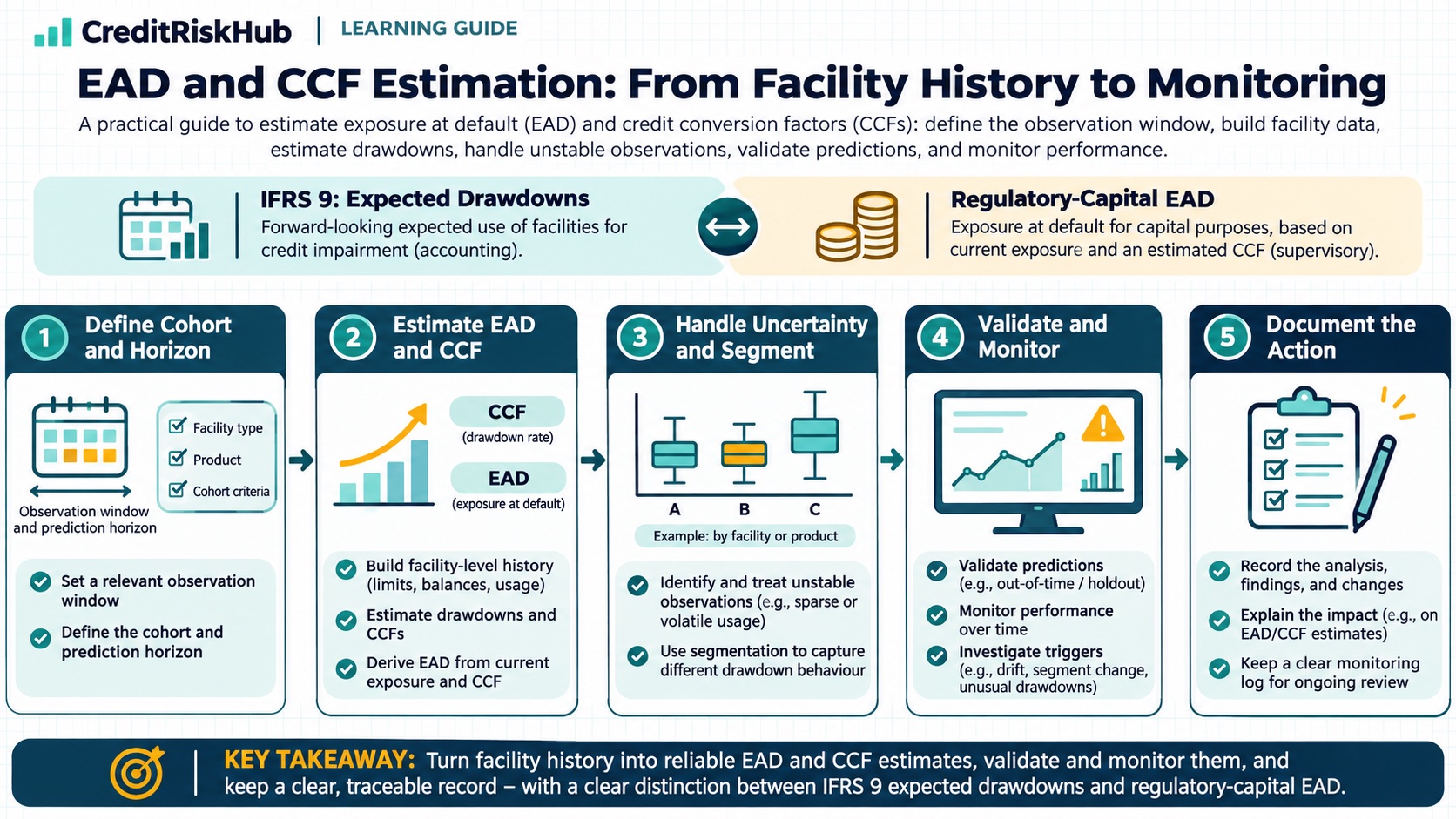
EAD and CCF Estimation: From Facility History to Monitoring

Exposure at default is the exposure expected to be outstanding when the relevant default event occurs. For a drawn balance plus an undrawn revolving amount, a simple representation is EAD = current drawn balance + expected additional drawings before or at default. A CCF expresses some form of expected future exposure as a fraction of a defined amount. The fraction depends on the chosen CCF convention; always label its numerator, denominator, and reference date.

For an undrawn-limit-factor (ULF) observation, let B0 be the facility balance at the reference date, L0 the applicable facility limit at that date, and BD the observed facility exposure at default. If unused capacity U0 = L0 − B0 is positive, the observed CCF can be calculated as CCF = (BD − B0) / (L0 − B0). The corresponding forecast under this convention is EAD-hat = Bt + CCF-hat × (Lt − Bt), where Bt and Lt are the drawn balance and usable limit at the forecast date. The forecast is only meaningful when the facility terms and limit definition match the history used to estimate CCF.

This is one modelling convention, not the definition of all EAD models. Basel’s IRB framework also describes limit-factor, balance-factor, and additional-utilisation approaches, and advanced-approach EAD may be estimated directly at facility level. Basel requires the estimate to reflect potential additional drawings up to and after a default trigger. Basel Framework CRE36.89–36.90 and CRE36.95 (https://www.bis.org/basel_framework/chapter/CRE/36.htm?inforce=20230101&published=20221208).

First define the unit of analysis: usually a facility, identified consistently across servicing, limit, and default systems. Set a default definition and date, decide whether the target is gross exposure or a specific accounting balance, and define how accrued interest, fees, over-limit amounts, repayments, restructures, and multiple facilities per borrower are treated. Keep those choices consistent from development through monitoring.

For Basel IRB EAD estimates, CRE36.93 specifies a 12-month fixed-horizon approach: each default outcome is linked to obligorA borrower or counterparty whose credit quality or default risk is assessed.Open full glossary entry ↗ and facility characteristics from twelve months before default. That is a regulatory requirement for the covered IRB use, not a universal window for every internal or accounting model. In other applications, choose a horizon that reflects the decision and expected exposure process, and validate that horizon explicitly. Basel Framework CRE36.93 (https://www.bis.org/basel_framework/chapter/CRE/36.htm?inforce=20230101&published=20221208).

Create one reference row per eligible facility-default event. Join the latest valid balance, contractual limit, facility status, product, grade, delinquency, and management state available at the reference date. Do not let information recorded after that date leak into predictors. Preserve limit histories and flag limit reductions, freezes, cancellations, product conversions, refinancing, and restructures. Those events can change both future drawing capacity and the meaning of the denominator.

Assume a revolving facility has a $100,000 limit and a $60,000 drawn balance twelve months before default. At default, the exposure is $82,000. Under the ULF convention, the unused amount at the reference date is $40,000, the net increase in exposure is $22,000, and the observed CCF is $22,000 / $40,000 = 55%. If a comparable facility today has a $100,000 usable limit and a $50,000 balance, applying a 55% estimate gives an illustrative EAD of $50,000 + 55% × $50,000 = $77,500.

Now consider an account that was already 98% utilized: a $100,000 limit, $98,000 drawn at the reference date, and $104,000 exposure at default. The same formula gives ($104,000 − $98,000) / ($100,000 − $98,000) = 300%. That observation is not automatically invalid. It is highly sensitive because the denominator is only $2,000, and the default exposure includes a $4,000 limit excess. Basel says EAD reference data should not be capped at principal or facility limits and should include accrued interest, other due payments, and limit excesses. It also cautions against treating CCFs above 100% or below zero by simply flooring/capping them or dropping affected observations. Basel Framework CRE36.95–36.96 (https://www.bis.org/basel_framework/chapter/CRE/36.htm?inforce=20230101&published=20221208).

This tiny example is not enough to estimate a portfolio parameter. It shows why a ratio can be unstable near full utilization, and why the bank should distinguish a real exposure process from bad joins or inconsistent limit units. A production policy might use another factor definition or a model that treats initial utilization as a driver. It should document the chosen method, preserve affected observations for analysis, and test how the choice changes predictions.

A robust pipeline starts with a default-event table and a dated facility snapshot. At minimum, retain facility and borrower identifiers, product and currency, default date and trigger, reference date, drawn exposure, contractual limit, amount actually available to draw, accrued interest and fees, facility status, payment state, internal grade, and limit-management actions. Keep source-system lineage so a reviewer can reproduce a row from the underlying ledger and contract history.

Use the contractual and operational amount that was available to the borrower at the reference date; do not assume the headline limit was fully drawable. Record conditions, borrowing bases, covenants, blocked drawdowns, and any control that materially constrains availability. Basel’s standardised CCF rules define which commitments are in scope for that approach, while its IRB standards require the bank to reflect its own monitoring, payment processing, and ability or willingness to prevent further drawings. The applicable rule depends on whether the calculation is standardised, IRB, accounting, or internal. Basel Framework CRE20.94 and CRE36.92 (https://www.bis.org/basel_framework/chapter/CRE/36.htm?inforce=20230101&published=20221208).

Run explicit data checks before calculating any factor. Confirm that facility identifiers resolve to one current contract, balance and limit dates use the same currency and unit, default dates are valid, and balances reconcile to ledger definitions. Investigate missing or negative limits, zero unused capacity, duplicate facility-default events, post-reference changes, and exposure values that appear truncated. Do not silently delete an observation simply because its CCF is inconvenient; classify the reason and quantify how exclusions or adjustments affect the result.

Start with economically meaningful facility groups: revolving versus term, product, retail versus commercial, secured versus unsecured when relevant, limit-utilization band, customer management strategy, and whether a line can actually be drawn during early arrears. Create a segment only when its contract and behavioural process differ enough to change exposure, and when the default sample supports a stable estimate. If the data are sparse, pool with a documented rationale or use a model that represents the driver continuously rather than combining unrelated products.

For an initial benchmark, calculate the observed CCF distribution and a clearly defined portfolio estimate. A simple arithmetic average gives each default event equal weight; a default-weighted EAD average gives more influence to exposures with larger balances. These answer different questions. For Basel advanced IRB corporate and sovereign own-EAD estimates, CRE36.98 specifies a default-weighted average and a minimum observation period; separate requirements apply to retail exposures. Follow the applicable paragraph and supervisory implementation rather than choosing a weighting by convenience. Basel Framework CRE36.98–36.99 (https://www.bis.org/basel_framework/chapter/CRE/36.htm?inforce=20230101&published=20221208).

A regression, tree-based model, or segmented factor can use reference-date drivers such as utilization, product, grade, line size, delinquency, and limit-management state. Train using only data available at the intended prediction time. A model should estimate exposure at default directly or estimate incremental drawings in a way that maps cleanly to the defined EAD. Compare it against a simple benchmark, inspect the predicted-versus-observed relationship across material groups, and explain how the model behaves near a full draw and around limit changes. More complexity is useful only if it improves reliable estimation and remains governable.

For IFRS 9, expected credit losses on undrawn loan commitments must be consistent with expected drawdowns. The standard’s application guidance distinguishes the portion expected to be drawn within twelve months for 12-month ECLThe portion of lifetime ECL associated with default events possible within the 12 months after the reporting date; it is not simply cash shortfalls occurring only in that year.Open full glossary entry ↗ from the portion expected over the expected life for lifetime ECLExpected credit losses resulting from all possible default events over the expected life of the financial instrument under applicable requirements.Open full glossary entry ↗. Specific combined loan-and-undrawn-commitment instruments can require measuring ECL over the period of credit-risk exposure even where that extends beyond the contractual cancellation notice period, when the conditions in IFRS 9 paragraph 5.5.20 apply. This is an accounting cash-shortfall estimate; it is not automatically the same target, horizon, or parameter as an IRB CCF. See IFRS 9 paragraphs B5.5.30–B5.5.31 and 5.5.20, summarized in this IFRS Foundation staff paper on revolving credit facilities (https://www.ifrs.org/content/dam/ifrs/meetings/2015/september/itg/impairment-of-financial-instruments/ap3-measurement-of-expected-credit-losses-for-revolving-credit-facilities.pdf).

Regulatory capital EAD follows the applicable prudential approach. Basel’s standardized approach applies supervisory CCFs to covered off-balance-sheet items. Under advanced IRB, eligible banks estimate EAD using the minimum requirements, including the relevant default horizon, representative data, and—where required—long-run default-weighted estimation, conservatism, and downturn treatment. An internal risk or pricing EAD can use a different horizon or objective, but it should be named and reconciled rather than presented as IFRS 9 or regulatory capital EAD. Basel Framework CRE32 and CRE36 (https://www.bis.org/basel_framework/chapter/CRE/36.htm?inforce=20230101&published=20221208).

Use a time-based holdout so the validation set reflects a later period than development. Keep all observations for the same borrower or connected group together where dependence would otherwise leak information across samples. Reconstruct every prediction using only data that would have been available at its reference date. Report results by product, utilization band, line size, rating, delinquency state, and material management-action groups; a strong portfolio average can hide substantial underprediction in a segment.

At portfolio level, compare predicted total EAD with realized total EAD. Define aggregate bias as (sum of predicted EAD − sum of realized EAD) / sum of realized EAD. A positive result indicates aggregate overprediction; a negative result indicates underprediction. Also calculate mean absolute error = average of |predicted EAD − realized EAD| and weighted absolute percentage error = sum of absolute errors / sum of realized EAD. Report the percentage of defaults where realized EAD exceeds the prediction as a diagnostic, not as a target that must be zero. For estimates intended to represent conditional means, evaluate calibrationAgreement between predicted probabilities and observed event frequencies for a matched population and horizon.Open full glossary entry ↗ and error by relevant groups; a high error rate may be expected when outcomes are variable, so interpret it alongside calibration and uncertainty.

Test robustness around near-full-utilization observations, over-limit balances, limit changes, and policy interventions. Compare the benchmark with alternatives such as a limit factor or direct EAD model, but do not use aggregate fit alone to choose. Check whether the result is driven by a handful of large exposures, one default vintage, or one operational rule. Document a decision log with data filters, definitions, observation window, weighting, model version, overlays, limitations, and approval.

Track realized-to-predicted EAD and aggregate bias by product and material segment. Review mean absolute error, weighted absolute percentage error, underprediction frequency, and the distribution of observed CCFs alongside predicted CCFs. Report default counts, exposure totals, confidence intervals or other uncertainty measures, and concentration in the largest obligors; do not interpret a percentage without its denominator.

Monitor input and process changes as well as model accuracy. Useful indicators include missing or stale limits, zero or negative available amounts, unexplained limit changes, share of exposures with restricted drawdown, line utilization distribution, product mix, delinquency mix, frequency of manual overrides, and shifts in default or collections policy. Basel requires EAD estimates to be reviewed when material information changes and at least annually across facility types, and requires daily monitoring of balances against commitments for banks under the specified IRB requirements. That does not mean every monitoring metric must be calculated daily; set frequency according to data availability, risk, and the governing policy. Basel Framework CRE36.91–36.93 (https://www.bis.org/basel_framework/chapter/CRE/36.htm?inforce=20230101&published=20221208).

Set escalation thresholds before looking at each month’s result. A practical trigger could combine material negative aggregate bias with enough defaults and exposure volume to make the finding meaningful, or trigger a review when input drift changes who can draw and how much. Assign an owner, investigation deadline, and actions such as data correction, segment review, recalibration, or formal model change. Keep the distinction between a temporary overlay and a rebuilt model clear in the governance record.

Using the limit at default instead of the limit at the reference date can create look-ahead bias and hide limit-management effects. Dividing by a very small unused amount can create extreme ratios; applying an arbitrary 0%–100% cap can erase real information. Mixing revolving credit cards, term loans, and facilities with different draw-stop policies can produce an average that describes none of them. Training on default-date attributes when the model is meant to predict twelve months earlier leaks the outcome into the predictors.

Another common mistake is treating IFRS 9 expected drawdowns, Basel standardized CCFs, advanced IRB own-EAD estimates, and internal planning forecasts as interchangeable. They may share exposure data while using different definitions, horizons, weighting, and policy objectives. Label each output, maintain reconciliations, and obtain accounting or regulatory interpretation for the applicable jurisdiction.

The worked facility balances and limits are synthetic and are for illustration only. The ULF formula assumes the same facility, compatible balance definitions, a positive unused amount at the reference date, and a limit that represents available credit under the chosen policy. Realized CCFs are noisy outcomes. The estimation method must account for portfolio heterogeneity, sampling uncertainty, limit changes, customer actions, and management interventions. The Basel requirements cited apply to the relevant Basel IRB framework; national rules and implementation dates can differ. This article is educational. It is not accounting, legal, or regulatory advice and does not define a bank’s approved EAD methodology.

Basel Committee on Banking Supervision, Basel Framework CRE32: IRB approach—risk components (https://www.bis.org/basel_framework/chapter/CRE/32.htm?inforce=20230101&published=20221208). Basel Committee on Banking Supervision, Basel Framework CRE36: IRB minimum requirements (https://www.bis.org/basel_framework/chapter/CRE/36.htm?inforce=20230101&published=20221208), especially CRE36.89–36.99. IFRS Foundation, ITG staff paper: Measurement of expected credit losses for revolving credit facilities (https://www.ifrs.org/content/dam/ifrs/meetings/2015/september/itg/impairment-of-financial-instruments/ap3-measurement-of-expected-credit-losses-for-revolving-credit-facilities.pdf), discussing IFRS 9 paragraphs B5.5.30–B5.5.31 and 5.5.20. The paper is explanatory staff material, not an IFRS requirement itself.

Educational material only. Confirm the governing accounting standard, prudential rules, model approval, and internal policy before using an EAD estimate in reporting, capital, or lending decisions.