Validation and governance

Reading PD Backtests When Defaults Are Rare

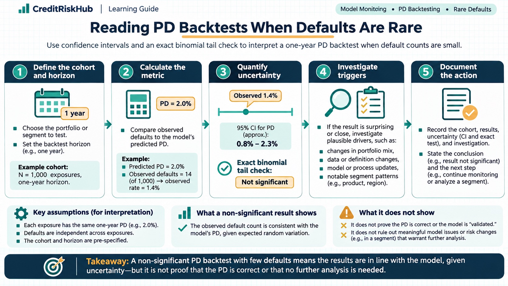
Use confidence intervals and an exact binomial tail check to interpret a one-year PD backtest when default counts are small. Learn the assumptions, calculate a synthetic example, and understand what a non-significant result does—and does not—show.

Updated 2026-10-24

A visual overview of Use confidence intervals and an exact binomial tail check to interpret a one-year PD backtest when default counts are small. Learn the assumptions, calculate a synthetic example, and understand what a non-significant result does—and does not—show. See the guide for assumptions and implementation details.

Purpose

Key terms

Hover over or focus a term for a quick definition, or open its glossary entry.

Formula

Expected defaults: 400 × 2% = 8.
Realised default rate: 13 / 400 = 3.25%.
O/E: 13 / 8 = 1.625.
European Banking Authority, Guidelines on PD estimation, LGD estimation and treatment of defaulted assets (EBA/GL/2017/16): https://eba.europa.eu/activities/single-rulebook/regulatory-activities/model-validation/guidelines-pd-estimation-lgd?version=2018

A low number of defaults can make a probability-of-default (PD) backtest hard to interpret. The observed default rate may be above the forecast simply because a small sample is noisy. It may also warn that the forecast is too low. A point estimate alone cannot distinguish those explanations.

This guide adds two diagnostics to a one-year, grade-level backtest: a Wilson confidence interval for the realised default rate and an exact, one-sided binomial test of whether the observed count is unusually high if the forecast PD were correct. They make sampling uncertainty visible. They do not certify a model or establish regulatory or accounting compliance.

DEFINITIONS

Forecast PD is the probability assigned to an obligor for a defined event and horizon. In this example it is a one-year probability. Realised default rate is defaults in the observation window divided by eligible obligors. It is an observed portfolio outcome, not an individual probability. Expected defaults under a common PD p and n eligible obligors is n × p. Observed-to-expected (O/E) is observed defaults divided by expected defaults; it is descriptive and does not express uncertainty by itself.

The Basel Committee distinguishes an ex-post default rate for a group from PD as a risk estimate. Its guidance warns that few loss events can make backtesting weak evidence about rating-system accuracy and recommends other validation evidence when data are scarce. Source: Basel Framework, Credit risk – internal ratings-based approach, section 30: https://www.bis.org/committees/bcbs/basel-consolidated-guidelines/module/cri/30

ASSUMPTIONS BEFORE CALCULATING

The binomial calculation treats each obligor outcome as an independent Bernoulli trial with the same one-year default probability. This is a useful teaching case for a reasonably homogeneous grade or pool, but real portfolios can violate both assumptions.

• Obligors can have different forecast PDs. Replacing them with the mean PD does not preserve the exact binomial distribution. For materially different PDs, consider a Poisson-binomial test or justified grouping.

• Defaults can be dependent because obligors share sectors, geographies, guarantors, or macroeconomic shocks. Dependence can make a simple binomial interval too narrow.

• Each account needs a complete, consistently defined one-year outcome window. Exclude or separately handle censored outcomes, changed eligibility, and inconsistent default definitions.

• Match the cohort’s observation date, default definition, rating assignment, and horizon to the forecast. Do not count overlapping windows as independent obligors.

These are model-validation diagnostics for forecast PDs. They are not IFRS 9 accounting expected credit loss (ECL), a Basel regulatory-capital calculation, or an internal pricing or risk-appetite measure. Those uses have different purposes, definitions, data requirements, and governance.

WORKED SYNTHETIC EXAMPLE

Suppose a grade contains 400 eligible obligors. Each has an illustrative one-year PD of 2%. Thirteen default during the fully matured one-year window.

The realised rate is above the forecast, but 13 events are still a small count. A Wilson 95% confidence interval is approximately 1.91% to 5.48%. It includes 2%, illustrating uncertainty; it does not prove the forecast is correct.

Under the common-PD binomial assumption, the exact one-sided probability of observing 13 or more defaults when n=400 and p=2% is approximately 6.19%. At a conventional 5% test level, this example does not reject that null hypothesis. That is not evidence the model is calibrated; it means this sample alone does not cross the chosen test threshold. The level is a diagnostic choice, not a universal supervisory threshold.

PYTHON EXAMPLE — SYNTHETIC AND BOUNDED

This uses only Python’s standard library and fixed inputs. It uses no randomness, external packages, network access, or customer data; the tail calculation is limited to at most 5,001 terms.

from math import exp, lgamma, log, log1p, sqrt

n = 400

observed_defaults = 13

forecast_pd = 0.02

confidence_z = 1.959963984540054 # two-sided 95% normal quantile

if not 1 <= n <= 5000:

raise ValueError("Use between 1 and 5,000 eligible obligors.")

if not 0 <= observed_defaults <= n:

raise ValueError("Observed defaults must be between zero and n.")

if not 0 < forecast_pd < 1:

raise ValueError("Forecast PD must be strictly between zero and one.")

observed_rate = observed_defaults / n

expected_defaults = n * forecast_pd

oe_ratio = observed_defaults / expected_defaults

# Wilson score interval for a binomial proportion.

z2 = confidence_z ** 2

denominator = 1 + z2 / n

center = (observed_rate + z2 / (2 * n)) / denominator

half_width = confidence_z * sqrt(

observed_rate * (1 - observed_rate) / n + z2 / (4 * n ** 2)

) / denominator

ci_low = max(0.0, center - half_width)

ci_high = min(1.0, center + half_width)

# Exact upper-tail probability P(X >= observed_defaults | n, forecast_pd).

def log_binomial_probability(x, trials, probability):

return (

lgamma(trials + 1)

- lgamma(x + 1)

- lgamma(trials - x + 1)

+ x * log(probability)

+ (trials - x) * log1p(-probability)

)

log_terms = [

log_binomial_probability(x, n, forecast_pd)

for x in range(observed_defaults, n + 1)

]

largest_log_term = max(log_terms)

upper_tail_probability = exp(largest_log_term) * sum(

exp(term - largest_log_term) for term in log_terms

)

upper_tail_probability = min(1.0, upper_tail_probability)

print(f"Eligible obligors: {n}")

print(f"Observed defaults: {observed_defaults}")

print(f"Expected defaults: {expected_defaults:.2f}")

print(f"Realised default rate: {observed_rate:.2%}")

print(f"Observed-to-expected: {oe_ratio:.3f}")

print(f"Wilson 95% interval: {ci_low:.2%} to {ci_high:.2%}")

print(f"Exact one-sided P(X >= observed): {upper_tail_probability:.2%}")

EXPECTED OUTPUT

Eligible obligors: 400

Observed defaults: 13

Expected defaults: 8.00

Realised default rate: 3.25%

Observed-to-expected: 1.625

Wilson 95% interval: 1.91% to 5.48%

Exact one-sided P(X >= observed): 6.19%

The one-sided test asks a narrow question: if every eligible obligor truly had the forecast 2% PD, how often would this cohort produce at least 13 defaults? It focuses on underprediction. A two-sided question would also count unusually few defaults and needs a separately specified test convention.

The Wilson interval estimates the cohort’s underlying event rate under a binomial sampling model. It is not a confidence interval for model parameters and does not account for regime shifts, dependence, selection effects, label errors, or misspecified PDs. NIST describes the Wilson interval as a binomial-proportion interval derived by inverting a hypothesis test: https://itl.nist.gov/div898/handbook/prc/section2/prc241.htm

PRACTICAL REVIEW WORKFLOW

1. Lock the population and horizon

Record the snapshot date, grade or pool, eligible obligors, default definition, maturity rule, and one-year outcome window.

2. Check counts before rates

Report n, observed defaults, expected defaults, realised rate, and O/E.

3. Show uncertainty

Include an interval and its assumptions. A wide interval in a low-default segment means the data have limited ability to distinguish plausible calibration levels.

4. Investigate causes

Review grade migration, risk mix, underwriting changes, macroeconomic conditions, data quality, default identification, and prior periods. Check whether results concentrate in a meaningful subsegment.

5. Use multiple validation lenses

Basel guidance discusses benchmarking, migration information, expert judgment, and broader portfolio outcomes where data are scarce. EBA guidance says realised rates should be compared with estimated PDs and deviations analysed in light of rating philosophy and economic conditions. Sources: EBA PD/LGD estimation guidelines https://eba.europa.eu/activities/single-rulebook/regulatory-activities/model-validation/guidelines-pd-estimation-lgd?version=2018 and PD calibration backtesting Q&A https://eba.europa.eu/single-rule-book-qa/qna/view/publicId/2023_6747

6. Set escalation rules before reviewing results

Define the test, confidence level, aggregation, review triggers, and actions in governance documentation. Avoid one p-value or generic O/E cutoff as an automatic model-approval rule.

7. Document conclusions proportionately

State what the evidence supports, what it cannot establish, and what additional data or analysis is needed. Failure to reject a null hypothesis is not proof of accuracy.

For portfolios with varying obligor PDs, compute the total-default distribution using a Poisson-binomial method or a documented simulation. If outcomes overlap or share material drivers, use a method that accounts for dependence. Do not claim regulatory compliance because the arithmetic is reproducible.

LIMITS AND INTERPRETATION

• A small p-value is a reason to investigate, not an automatic instruction to recalibrate. Check population construction, default timing, data quality, and risk mix.

• A large p-value can reflect low power; it does not confirm the model.

• Repeated tests across grades, months, and segments raise the chance of apparently unusual results. Document the test set and monitoring design.

• Observed rates can move with the business cycle while long-run calibration asks a different question. State whether the model is point-in-time or through-the-cycle.

• Regulatory backtesting and disclosures have specific definitions. Internal monitoring does not replace applicable requirements.

REFERENCES

Basel Committee, Credit risk – internal ratings-based approach, sections 30.56–30.72: https://www.bis.org/committees/bcbs/basel-consolidated-guidelines/module/cri/30

European Banking Authority, Q&A 2023_6747, PD calibration sample: https://eba.europa.eu/single-rule-book-qa/qna/view/publicId/2023_6747

NIST/SEMATECH e-Handbook, confidence intervals for proportions: https://itl.nist.gov/div898/handbook/prc/section2/prc241.htm

SciPy binomtest documentation (reference only; this example uses the standard library): https://docs.scipy.org/doc/scipy/reference/generated/scipy.stats.binomtest.html

Educational example only. All values are synthetic. This statistical diagnostic is not accounting, regulatory, or legal advice. Validate assumptions, definitions, and governance requirements for the intended portfolio and use.

Try a reproducible Python example

These examples use synthetic inputs and run locally in a browser worker. Edit the code, run it, and compare its output with the published example.

Runnable Python · local in your browser

Monitor observed-to-expected and Brier score

Compare a small set of matured binary outcomes against predicted PD values.

Editable Python example

Output

Run the code to see the output.

Runtime loads only after you press Run. Code runs in a separate browser worker with a 10-second limit and a 20,000-character output cap. Use synthetic examples only; browser execution is not a secure environment for secrets or sensitive records.

Runnable Python · local in your browser

Calculate ROC-AUC, Gini, KS, precision, and recall

Use synthetic out-of-sample scores and matured labels. Higher scores indicate higher risk; the example computes pairwise ROC-AUC and a threshold-specific operating point.

Editable Python example

scores = [0.92, 0.81, 0.65, 0.58, 0.42, 0.20]
observed_default = [1, 1, 1, 0, 0, 0]
positives = [score for score, y in zip(scores, observed_default) if y == 1]
negatives = [score for score, y in zip(scores, observed_default) if y == 0]
pairs = [(bad, good) for bad in positives for good in negatives]
auc = sum(1 if bad > good else 0.5 if bad == good else 0 for bad, good in pairs) / len(pairs)
gini = 2 * auc - 1
threshold = 0.60
tp = sum(y == 1 and score >= threshold for score, y in zip(scores, observed_default))
fp = sum(y == 0 and score >= threshold for score, y in zip(scores, observed_default))
fn = sum(y == 1 and score < threshold for score, y in zip(scores, observed_default))
precision = tp / (tp + fp) if tp + fp else 0
recall = tp / (tp + fn) if tp + fn else 0
ks = max(abs(sum(y == 1 and score >= cut for score, y in zip(scores, observed_default)) / len(positives) - sum(y == 0 and score >= cut for score, y in zip(scores, observed_default)) / len(negatives)) for cut in scores)
print(f"ROC-AUC={auc:.3f}; Gini={gini:.3f}; KS={ks:.3f}")
print(f"At threshold {threshold:.2f}: precision={precision:.3f}; recall={recall:.3f}")

Output

Run the code to see the output.

References

Basel Committee; European Banking Authority; NIST — Basel Committee; European Banking Authority; NIST

Educational material only. Methods and examples are simplified; state and validate the assumptions required for your use case.