Validation and governance

How to Compare Two PD Models with a Paired Bootstrap

Compare discrimination from two PD models on the same matured validation cohort with a paired, stratified bootstrap confidence interval for the AUC difference.

Updated 2026-11-01

Visual summary: How to Compare Two PD Models with a Paired Bootstrap.

Purpose

Compare discrimination from two PD models on the same matured validation cohort with a paired, stratified bootstrap confidence interval for the AUC difference.

Key terms

Hover over or focus a term for a quick definition, or open its glossary entry.

Formula

Primary statistic: Challenger minus incumbent, ΔAUC = AUC_B − AUC_A.
AUC = P(score_default > score_nondefault) + 0.5 × P(tie)
AUC difference = AUC_B − AUC_A
There are 8 × 24 = 192 default/non-default pairs. Count a pair as correctly ranked when the default score is higher; a tie counts as one-half.
Model A: 143.5 correctly ranked pair-equivalents ÷ 192 pairs = AUC 0.7474.
Model B: 164 correctly ranked pair-equivalents ÷ 192 pairs = AUC 0.8542.
AUC difference = 0.8542 − 0.7474 = 0.1068
95% percentile interval = [quantile(ΔAUC*, 0.025), quantile(ΔAUC*, 0.975)]

A model with a higher area under the ROC curve (ROC-AUC) may rank defaults better, but is the difference larger than sampling noise? When two probability-of-default (PD) models score the same borrowers, their AUC estimates are paired. Resampling the borrower records together preserves that pairing.

This guide compares two fixed models on the same fully matured validation cohort using a paired, stratified bootstrap confidence interval for the AUC difference. All observations and scores are synthetic. The tiny example is for learning and is not enough to support a production model decision.

SCOPE

This is a statistical validation diagnostic for rank discrimination. It is not an IFRS 9 expected credit loss calculation, a Basel regulatory-capital calculation, a calibration test, or a business-impact analysis.

PAIRED AUC COMPARISON AT A GLANCE

Question: Which models? Incumbent A and challenger B, both scored on the same borrowers and outcomes.

Why paired? Each sampled borrower contributes the same outcome and both model scores to each bootstrap replicate.

Interval interpretation: Sampling variation under the specified resampling scheme, conditional on this cohort and its observed number of defaults and non-defaults.

Not established: Calibration, causal benefit, training stability, regulatory approval, or better customer outcomes.

1. DEFINE THE COMPARISON BEFORE CALCULATING

1. Define one matured cohort

Record the score date, default definition, performance horizon, eligibility rules, and data cut-off. Include only accounts whose outcome is fully observed for the horizon, or specify how censoring and missing outcomes are handled.

2. Freeze predictions from both models

Confirm that neither model used validation outcomes or post-score information. Record model versions, feature cut-offs, and score transformations.

3. Set score direction

In this example, larger scores mean higher default risk. A strictly increasing transformation preserves AUC; reversing score direction reverses its interpretation.

4. Choose the estimand

We measure challenger-minus-incumbent AUC. A positive estimate favours B on ranking in this sample, but does not alone justify replacing A.

5. Pre-specify the uncertainty method and interval

DeLong's method is a common analytic approach for correlated ROC curves; a paired bootstrap is an approachable resampling alternative. Choose based on the cohort and design, not on which result looks preferable.

The outcome horizon must match the intended PD target. A 12-month default label is not interchangeable with a lifetime-default label. See the CreditRiskHub glossary entries for probability of default and backtesting.

2. WHAT AUC AND THE DIFFERENCE MEAN

ROC-AUC can be interpreted as the probability that a randomly selected default receives a higher risk score than a randomly selected non-default, with half-credit for a tie.

For challenger B and incumbent A, define:

AUC measures ranking, not probability accuracy. A model can rank borrowers well while its predicted PDs are systematically too high or too low. Assess calibration separately.

3. SYNTHETIC WORKED EXAMPLE

There are 32 synthetic borrowers: 8 defaults and 24 non-defaults. Both fixed models have a score for every borrower. A larger value means higher risk.

Default scores — Model A: 0.90, 0.84, 0.74, 0.63, 0.52, 0.45, 0.35, 0.20

Default scores — Model B: 0.95, 0.90, 0.84, 0.78, 0.71, 0.65, 0.49, 0.40

Non-default scores — Model A: 0.95, 0.80, 0.70, 0.65, 0.60, 0.55, 0.50, 0.45, 0.40, 0.38, 0.35, 0.33, 0.30, 0.28, 0.25, 0.23, 0.20, 0.18, 0.15, 0.12, 0.10, 0.08, 0.05, 0.02

Non-default scores — Model B: 0.92, 0.80, 0.72, 0.68, 0.63, 0.59, 0.52, 0.46, 0.44, 0.41, 0.37, 0.34, 0.30, 0.27, 0.24, 0.22, 0.19, 0.16, 0.13, 0.11, 0.09, 0.06, 0.03, 0.01

In this constructed sample, B ranks defaults above non-defaults more often. The interval below shows how the difference varies when we repeatedly resample this cohort.

4. PAIRED, STRATIFIED BOOTSTRAP: SIX STEPS

1. Separate borrower indices into defaults and non-defaults

2. In each replicate, sample 8 default indices with replacement from the 8 defaults, and 24 non-default indices with replacement from the 24 non-defaults

3. Combine the sampled indices

Use that exact same index list to select both A's and B's scores. This preserves pairing.

4. Recalculate AUC_A, AUC_B, and ΔAUC for the replicate

5. Repeat a pre-specified number of times with a recorded random seed

6. Sort the replicate differences

The 2.5th and 97.5th percentiles form a percentile 95% interval in this teaching example.

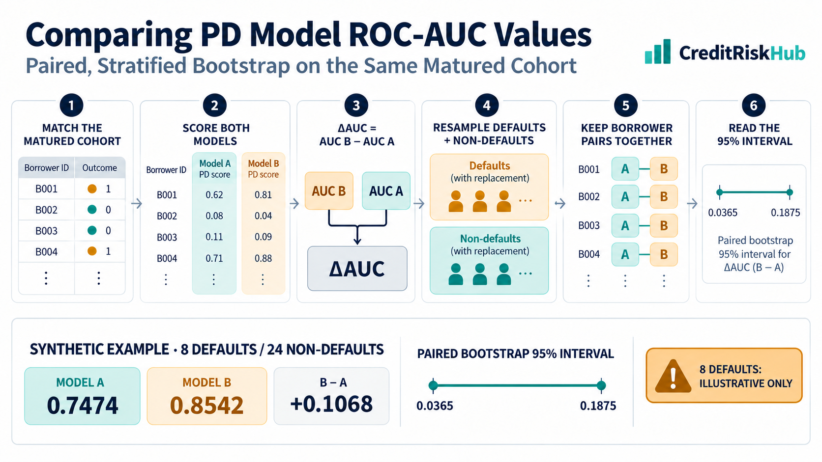
Workflow infographic: MATCH THE MATURED COHORT → CALCULATE BOTH AUCs → SUBTRACT B − A → RESAMPLE EACH OUTCOME CLASS → KEEP BORROWERS PAIRED → INTERPRET THE INTERVAL WITH EVENT COUNTS.

The interval summarizes variation under this resampling scheme and its assumptions. It is not a statement that a fixed model has a 95% chance of being better.

5. RESULT AND INTERPRETATION

Using 2,000 replicates and random seed 20261031, the paired stratified percentile interval is approximately 0.0365 to 0.1875.

Incumbent A ROC-AUC: 0.7474 — ranking on the synthetic cohort.

Challenger B ROC-AUC: 0.8542 — ranking on the same cohort.

Difference, B − A: 0.1068 — observed difference in this sample.

Paired bootstrap 95% percentile interval: 0.0365 to 0.1875 — resampling uncertainty conditional on these class counts and this cohort.

Although the lower endpoint is above zero here, only eight defaults make the bootstrap distribution coarse and unstable. The data are artificial and the interval captures only one source of uncertainty. This is a demonstration of mechanics, not evidence to approve a model.

6. IMPLEMENTATION CHECKLIST

1. Validate the input: one row per independent unit, same matured outcome and horizon, and one score from each model

2. Check that both outcome classes are present and that higher scores consistently mean higher risk

3. Calculate both AUCs on the original cohort and the paired difference

4. Resample borrower indices within outcome classes

Apply each sampled index to the labels and both score arrays.

5. Record the seed, number of replicates, quantile convention, cohort dates, event counts, and software version

6. Review the interval alongside the individual AUCs and other validation evidence

Keep code, data definitions, and model versions reproducible.

For a production implementation, use a reviewed statistical library, verify tie handling and quantile convention, and test against a known example. Pairwise AUC calculation is simple for this small example but can be inefficient on large datasets.

7. ASSUMPTIONS, MONITORING, AND WHEN TO CHANGE THE METHOD

Matched predictions: every row must refer to the same borrower, outcome, horizon, and eligibility under both models. If not, rebuild a matched cohort; do not call an unmatched comparison paired.

Mature outcomes: each label must have the full performance period to resolve. Otherwise exclude immature records or use a justified method for censoring.

Independent unit: repeated accounts from one borrower are dependent. Resample at borrower level; consider cluster or time-block resampling when observations share dependencies.

Rare defaults: every replicate must contain both classes. Stratification preserves observed class counts, but does not create information. A tiny default count still produces a coarse, unstable interval; collect more mature evidence where possible.

Fixed predictions: this bootstrap measures evaluation-sample uncertainty for these trained models. It does not rerun feature selection, tuning, or fitting. Use repeated development samples or nested resampling if training and model-selection variability is the question.

AUC is the right objective: also assess calibration, stability, segment performance, operational constraints, and decision impact.

Monitor both AUCs, their paired difference and interval, event/non-event counts, cohort dates, score direction, and outcome maturity on pre-defined windows. Avoid reacting to noisy monthly changes when defaults are sparse. Set thresholds based on intended use, portfolio, and governance policy; there is no universal acceptable AUC-difference threshold.

If borrowers recur across periods, ordinary row-wise resampling treats correlated observations as independent and may understate uncertainty. If the decision concerns future economic conditions, retain a genuine out-of-time holdout; random resampling does not reproduce regime change.

8. WHAT THIS COMPARISON DOES NOT TELL YOU

Calibration: ranking can be strong while PD values are too high or low. Review calibration plots, observed-to-expected ratios, calibration intercept and slope, and suitable uncertainty measures separately.

Training uncertainty: resampling fixed predictions does not repeat feature selection, model fitting, tuning, or governance decisions.

Subgroup performance: aggregate AUC can conceal poor ranking or instability in a relevant segment. Review justified segments with adequate data and governance safeguards.

Business value: higher AUC does not automatically improve approvals, pricing, losses, customer outcomes, or profit. Evaluate decisions and consequences separately.

Accounting and regulatory measures: AUC does not calculate IFRS 9 ECL, Basel capital, or internal risk appetite. These have distinct objectives, definitions, horizons, and governance.

If an interval crosses zero, this method and sample do not clearly resolve the direction; that does not prove equivalence. If the interval excludes zero, the result is still one part of model validation, not an automatic replacement decision.

REFERENCES

DeLong, DeLong & Clarke-Pearson (1988), Comparing the areas under two or more correlated receiver operating characteristic curves: a nonparametric approach. https://pubmed.ncbi.nlm.nih.gov/3203132/

Zhang et al. (2020), Confidence intervals of the difference between areas under two ROC curves in matched-pair experiments. https://doi.org/10.1002/sim.8562

scikit-learn, roc_auc_score documentation. https://scikit-learn.org/stable/modules/generated/sklearn.metrics.roc_auc_score.html

Basel Framework CRE 36: IRB approach, validation. This reference applies within its IRB scope and does not prescribe this bootstrap for all model comparisons. https://www.bis.org/basel_framework/chapter/CRE/36/inforce/2023-01-01/published/2020-03-27

CreditRiskHub glossary: https://creditriskhub.com/glossary

Educational illustration only. All observations and scores are synthetic. This is not investment, accounting, regulatory, or model-approval advice. Select and document methods for the cohort, dependence structure, event count, model use, and applicable governance requirements.

Try a reproducible Python example

These examples use synthetic inputs and run locally in a browser worker. Edit the code, run it, and compare its output with the published example.

Runnable Python · local in your browser

Monitor observed-to-expected and Brier score

Compare a small set of matured binary outcomes against predicted PD values.

Editable Python example

Output

Run the code to see the output.

Runtime loads only after you press Run. Code runs in a separate browser worker with a 10-second limit and a 20,000-character output cap. Use synthetic examples only; browser execution is not a secure environment for secrets or sensitive records.

Runnable Python · local in your browser

Calculate ROC-AUC, Gini, KS, precision, and recall

Use synthetic out-of-sample scores and matured labels. Higher scores indicate higher risk; the example computes pairwise ROC-AUC and a threshold-specific operating point.

Editable Python example

scores = [0.92, 0.81, 0.65, 0.58, 0.42, 0.20]
observed_default = [1, 1, 1, 0, 0, 0]
positives = [score for score, y in zip(scores, observed_default) if y == 1]
negatives = [score for score, y in zip(scores, observed_default) if y == 0]
pairs = [(bad, good) for bad in positives for good in negatives]
auc = sum(1 if bad > good else 0.5 if bad == good else 0 for bad, good in pairs) / len(pairs)
gini = 2 * auc - 1
threshold = 0.60
tp = sum(y == 1 and score >= threshold for score, y in zip(scores, observed_default))
fp = sum(y == 0 and score >= threshold for score, y in zip(scores, observed_default))
fn = sum(y == 1 and score < threshold for score, y in zip(scores, observed_default))
precision = tp / (tp + fp) if tp + fp else 0
recall = tp / (tp + fn) if tp + fn else 0
ks = max(abs(sum(y == 1 and score >= cut for score, y in zip(scores, observed_default)) / len(positives) - sum(y == 0 and score >= cut for score, y in zip(scores, observed_default)) / len(negatives)) for cut in scores)
print(f"ROC-AUC={auc:.3f}; Gini={gini:.3f}; KS={ks:.3f}")
print(f"At threshold {threshold:.2f}: precision={precision:.3f}; recall={recall:.3f}")

Output

Run the code to see the output.

References

DeLong, DeLong & Clarke-Pearson (1988), Biometrics — DeLong, DeLong & Clarke-Pearson (1988), Biometrics

Educational material only. Methods and examples are simplified; state and validate the assumptions required for your use case.