Validation and governance

A Step-by-Step Credit Risk Model Monitoring Framework

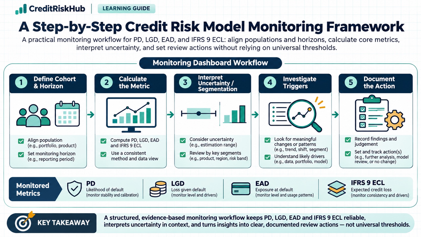
A practical monitoring workflow for PD, LGD, EAD, and IFRS 9 ECL: align populations and horizons, calculate core metrics, interpret uncertainty, and set review actions without relying on universal thresholds.

Updated 2026-10-25

A visual overview of A practical monitoring workflow for PD, LGD, EAD, and IFRS 9 ECL: align populations and horizons, calculate core metrics, interpret uncertainty, and set review actions without relying on universal thresholds. See the guide for assumptions and implementation details.

Purpose

Key terms

Hover over or focus a term for a quick definition, or open its glossary entry.

Formula

• Observed-to-expected (O/E) = sum(yᵢ) / sum(pᵢ). It compares total defaults with total forecast defaults. O/E above one means more defaults occurred than predicted in that cohort; below one means fewer occurred. Show counts and uncertainty: a ratio can be unstable when expected defaults are very small.
• Brier score = mean((yᵢ − pᵢ)²). Lower is better for the evaluated sample, but it depends on event prevalence and does not identify whether error came from ranking or calibration. Log loss = −mean(yᵢ ln(pᵢ) + (1−yᵢ) ln(1−pᵢ)); it penalizes confident errors strongly, so validate probability bounds and data quality first.
Suppose a matured cohort has 1,000 eligible obligors, 20 observed defaults, and a sum of forecast one-year PDs of 15. The realised rate is 20 / 1,000 = 2.0%; expected defaults are 15; O/E is 20 / 15 = 1.33. This is a signal to investigate and compare uncertainty, mix, prior periods, and segments. It is not by itself proof that the PD model is wrong, nor an automatic recalibration rule.
Basel Framework, CRE 36 — IRB approach minimum requirements, including review of estimates, appropriate data, and EAD monitoring: https://www.bis.org/basel_framework/chapter/CRE/36.htm?inforce=20230101&published=20200327
Basel Framework, CRE 30 — IRB overview and risk-component context: https://www.bis.org/basel_framework/chapter/CRE/30.htm?inforce=20230101&published=20200327
European Banking Authority, Guidelines on PD estimation, LGD estimation and treatment of defaulted assets (EBA/GL/2017/16); applicable to its defined EU IRB scope: https://eba.europa.eu/activities/single-rulebook/regulatory-activities/model-validation/guidelines-pd-estimation-lgd?version=2018
IFRS 9, especially paragraphs 5.5.17 and B5.5.28: https://www.ifrs.org/content/dam/ifrs/publications/pdf-standards/english/2022/issued/part-a/ifrs-9-financial-instruments.pdf?bypass=on

PURPOSE

Model monitoring is a controlled comparison between what a credit-risk model predicted, what the data and process actually produced, and what the model is intended to measure. A useful monitoring pack combines data and implementation checks, population stability, outcome performance, and governance review. No single metric can establish that a model remains fit for use.

This guide provides a repeatable workflow across scorecards, probability of default (PD), loss given default (LGD), exposure at default (EAD), and IFRS 9 expected credit losses (ECL). It is educational. Basel IRB requirements apply to banks and portfolios within their regulatory scope; IFRS 9 measurement is an accounting exercise under an entity’s applicable reporting framework. Internal risk monitoring has its own intended use and thresholds.

STEP 1 — STATE THE MODEL’S PURPOSE AND TARGET

For every model, record its owner, version, intended decisions, population, unit of analysis, target, default or loss definition, measurement date, forecast horizon, and update frequency. Say whether a PD is point-in-time or through-the-cycle and whether it is a regulatory estimate, an accounting input, or an internal risk measure. Do not compare estimates to outcomes with a different definition or purpose.

STEP 2 — FREEZE THE COHORT AND MATURED OUTCOME WINDOW

Create a reproducible snapshot of exposures eligible at the forecast date. Match each forecast with the outcome window it was meant to predict. Mark incomplete outcomes as immature or censored; do not label them non-default merely because default has not happened yet. For repeated records, use consistent obligor and facility keys and prevent one customer from leaking across development and validation samples. Record exclusions, missing labels, joins, and any changes in servicing or recovery practice.

STEP 3 — CHECK DATA AND IMPLEMENTATION BEFORE MODEL SCORES

Compare production inputs with their approved definitions: missingness, invalid values, category mapping, range violations, duplicates, date coverage, join rates, and feature availability at the forecast date. Reconcile a sample from source systems through transformations to the final score and decision. Verify model version, coefficient or tree artifact, calibration, cut-offs, overrides, and downstream use. A healthy performance metric cannot compensate for incorrect data or a production implementation mismatch.

STEP 4 — MONITOR POPULATION AND FEATURE STABILITY

Compare current inputs and score distributions with a fixed, documented reference population, using stable bins and consistent weights. One common Population Stability Index is PSI = sum over bins of (current share − reference share) × ln(current share / reference share). If a share is zero, use a documented small-value smoothing rule so the logarithm is defined, and report that choice. Feature stability can be assessed in the same way, alongside missingness, category novelty, range shifts, and changes in portfolio mix.

A stability index is a screening signal; it does not show that risk ranking or calibration has deteriorated. Investigate which segments or inputs moved, why they moved, whether the shift is expected, and whether the reference remains relevant. There is no universal PSI alert value suitable for every model and portfolio.

STEP 5 — ASSESS PD MODEL PERFORMANCE ON MATURED OUTCOMES

For binary outcomes yᵢ (1 for default, 0 otherwise) and forecasts pᵢ, report the sample size, default count, forecast horizon, and segment coverage before interpreting a ratio or score.

• Calibration by band compares average forecast PD with the observed default frequency within groups. Publish band definitions, counts, matured default counts, and confidence intervals. A whole-portfolio match can hide offsetting underprediction and overprediction across grades, vintages, products, or geographies.

• ROC-AUC measures how often a randomly selected defaulter is ranked above a randomly selected non-defaulter, with a half credit for ties. Gini = 2 × AUC − 1 under this convention. KS is the maximum separation between cumulative score distributions of defaulters and non-defaulters. For rare defaults, include precision-recall measures and the baseline default prevalence; accuracy alone can look high when almost all observations are non-defaults.

Discrimination metrics measure ranking, not probability calibration or business value. Compare metrics using the same outcome horizon, sample definition, and weighting. Report uncertainty and segment results; avoid implying a universal minimum AUC or maximum error applies to every use.

STEP 6 — REVIEW SCORECARD AND DECISION OUTCOMES

Track score distribution, grade migration, approval and decline rates, override frequency and direction, rank ordering, observed bad rates by score band, and outcome maturity. Separate population changes from policy changes: a new cut-off or strategy can alter which applicants receive a loan, making later outcome comparisons subject to selection effects. Monitor rejected applicants only when a valid outcome source and defensible method exist; do not imply their outcomes are directly observed when they are not.

STEP 7 — VALIDATE LGD AND RECOVERY OUTCOMES

Define the recovery cohort and when recoveries are considered complete. A simple realised economic LGD for a closed workout can be expressed as (EAD at default − present value of net recoveries) / EAD at default. Net recoveries should reflect relevant direct costs, timing, collateral proceeds, and discounting under the model’s defined methodology. Compare predicted and realised LGD by product, security, seniority, geography, workout status, and default vintage where sample size allows.

Report exposure-weighted average error, signed bias, absolute error, and predicted-versus-realised summaries alongside counts and unresolved-workout shares. Recoveries can take years; immature cases and changed collection practices can distort short-window comparisons. Basel IRB downturn LGD and regulatory conservatism are specific prudential concepts, not automatically the same as accounting ECL assumptions.

STEP 8 — VALIDATE EAD AND CONVERSION FACTORS

EAD is the gross exposure expected at default under a stated definition and horizon. For undrawn commitments, a credit conversion factor (CCF) relates the increase in drawn exposure before default to the relevant undrawn amount, subject to the applicable methodology. Compare forecast EAD with observed exposure at default on matched facilities and a fixed horizon. Report signed bias, mean or exposure-weighted absolute error, and results by product, commitment type, utilization, and risk segment.

Avoid relying on percentage error when the denominator can be close to zero. Show counts, exposure weights, and the distribution of errors. Reconcile limits, current drawn balances, cancelled commitments, repayments, and facility identifiers. Regulatory own-EAD estimation has specific Basel minimum requirements; internal forecasting and accounting uses may differ.

STEP 9 — REVIEW IFRS 9 ECL AS AN ACCOUNTING ESTIMATE

IFRS 9 ECL is a probability-weighted present value of cash shortfalls that reflects time value of money and reasonable, supportable information about past events, current conditions, and forecasts. Twelve-month ECL is the lifetime cash shortfall associated with default events possible in the 12 months after the reporting date; it is not simply the cash shortfall expected to occur during those 12 months.

Monitor stage allocation and significant-increase-in-credit-risk logic, scenario definitions and weights, forecast-to-realized drivers, PD/LGD/EAD inputs, discounting, write-offs, modifications, and reconciliations to the ledger. For backtesting, align the forecast cohort, reporting date, cash-flow definition, observation period, and scenario assumptions to the realized outcome being assessed. Decompose differences into volume and mix, staging, scenario, model parameter, data, and post-model adjustment effects. Lifetime loss outcomes may not yet be fully observed; label incomplete comparisons and do not treat realized one-year defaults as a direct substitute for lifetime ECL.

Keep IFRS 9 impairment ECL separate from Basel regulatory expected loss/capital and internal pricing or risk appetite measures. Similar labels do not make the measures interchangeable.

STEP 10 — TURN SIGNALS INTO REVIEW ACTIONS

Set monitoring frequency and escalation rules before results arrive. Base them on materiality, model use, portfolio size, uncertainty, data availability, and the consequences of an error. When a signal breaches an approved rule, validate the underlying data and implementation, identify affected segments, compare with external or challenger evidence where appropriate, assess customer and financial impacts, and document the owner and deadline for action. A threshold is an investigation trigger, not an automatic instruction to recalibrate or disable a model.

Record the evidence, limitations, decision, approval, remediation, and follow-up date. Keep versioned definitions, code, data snapshots or reproducible extracts, model artifacts, and monitoring outputs so an independent reviewer can reproduce the result. Reassess the monitoring design when the portfolio, policy, economic regime, or model use changes.

SYNTHETIC PD EXAMPLE

PRACTICAL MONITORING CHECKLIST

1. Confirm purpose, version, population, target, horizon, and reporting date. 2. Reconcile source data, joins, outcome maturity, and production implementation. 3. Show portfolio and feature stability with the reference population and binning rules. 4. Report outcome counts and uncertainty before PD performance ratios or scores. 5. Review ranking, calibration, scorecard decisions, override patterns, LGD recoveries, EAD, and ECL through measures appropriate to each target. 6. Segment results only where definitions are consistent and samples support interpretation; disclose low-default and immature groups. 7. Compare with development baselines, prior periods, challengers, and external evidence where relevant. 8. Apply documented escalation, investigate causes, and record an accountable action and review date.

REFERENCES

Educational material only. Values are synthetic. Metric definitions, denominators, observation windows, discounting, and governance must be validated for the intended portfolio and applicable accounting or regulatory framework.

Try a reproducible Python example

These examples use synthetic inputs and run locally in a browser worker. Edit the code, run it, and compare its output with the published example.

Runnable Python · local in your browser

Monitor observed-to-expected and Brier score

Compare a small set of matured binary outcomes against predicted PD values.

Editable Python example

Output

Run the code to see the output.

Runtime loads only after you press Run. Code runs in a separate browser worker with a 10-second limit and a 20,000-character output cap. Use synthetic examples only; browser execution is not a secure environment for secrets or sensitive records.

Runnable Python · local in your browser

Calculate ROC-AUC, Gini, KS, precision, and recall

Use synthetic out-of-sample scores and matured labels. Higher scores indicate higher risk; the example computes pairwise ROC-AUC and a threshold-specific operating point.

Editable Python example

scores = [0.92, 0.81, 0.65, 0.58, 0.42, 0.20]
observed_default = [1, 1, 1, 0, 0, 0]
positives = [score for score, y in zip(scores, observed_default) if y == 1]
negatives = [score for score, y in zip(scores, observed_default) if y == 0]
pairs = [(bad, good) for bad in positives for good in negatives]
auc = sum(1 if bad > good else 0.5 if bad == good else 0 for bad, good in pairs) / len(pairs)
gini = 2 * auc - 1
threshold = 0.60
tp = sum(y == 1 and score >= threshold for score, y in zip(scores, observed_default))
fp = sum(y == 0 and score >= threshold for score, y in zip(scores, observed_default))
fn = sum(y == 1 and score < threshold for score, y in zip(scores, observed_default))
precision = tp / (tp + fp) if tp + fp else 0
recall = tp / (tp + fn) if tp + fn else 0
ks = max(abs(sum(y == 1 and score >= cut for score, y in zip(scores, observed_default)) / len(positives) - sum(y == 0 and score >= cut for score, y in zip(scores, observed_default)) / len(negatives)) for cut in scores)
print(f"ROC-AUC={auc:.3f}; Gini={gini:.3f}; KS={ks:.3f}")
print(f"At threshold {threshold:.2f}: precision={precision:.3f}; recall={recall:.3f}")

Output

Run the code to see the output.

References

Basel Committee; European Banking Authority; IFRS Foundation — Basel Committee; European Banking Authority; IFRS Foundation

Educational material only. Methods and examples are simplified; state and validate the assumptions required for your use case.