Credit risk foundations
Expected loss and uncertainty
Calculate the loss average, quantify dispersion, and see why equal expected losses can hide different outcomes.
Purpose
Build a probability-weighted loss distribution, compare its mean and spread, and decide what additional portfolio monitoring is needed.
Key terms
Hover over or focus a term for a quick definition, or open its glossary entry.
Key definitions
- Expected loss is the probability-weighted average of loss outcomes for a defined unit and horizon.
- Variance and standard deviation summarize dispersion around the mean; neither is a complete description of tail risk.
E[L] = Σᵢ pᵢLᵢ
Var(L) = Σᵢ pᵢ(Lᵢ − E[L])²
σ(L) = √Var(L)
Var(Σⱼ Lⱼ) = Σⱼ Var(Lⱼ) + 2Σⱼₖ Cov(Lⱼ, Lₖ), for j < k
Worked example
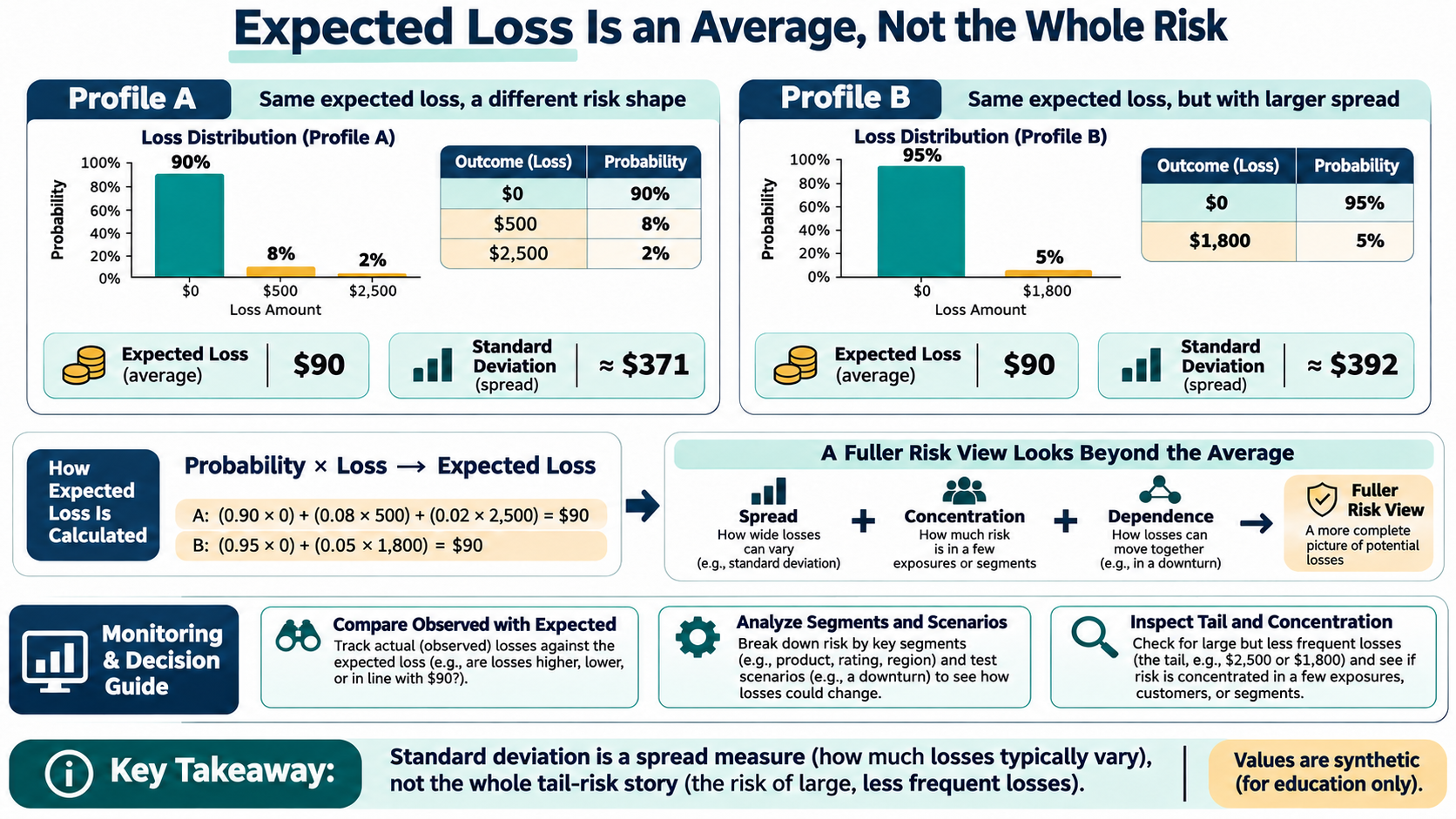
Two synthetic portfolios each have expected loss $90. Portfolio A has a 90% chance of $0 loss, 8% chance of $500, and 2% chance of $2,500: expected loss = $90 and standard deviation ≈ $371. Portfolio B has a 95% chance of $0 loss and 5% chance of $1,800: expected loss = $90 and standard deviation ≈ $392. The averages match, but the possible loss patterns differ.
| Profile / outcome | Probability | Loss | Contribution to mean |
|---|---|---|---|
| A: no loss | 90% | $0 | $0 |
| A: moderate loss | 8% | $500 | $40 |
| A: large loss | 2% | $2,500 | $50 |
| B: no loss | 95% | $0 | $0 |
| B: loss | 5% | $1,800 | $90 |
| View | Example measure | Interpretation / caution |
|---|---|---|
| Average calibration | Observed loss ÷ expected loss | Align cohort, horizon, loss definition and maturity; low counts are noisy. |
| Severity and timing | Recovery rate, workout duration, loss severity | Changes can arise from collateral mix, costs, or delayed recoveries. |
| Concentration | Top obligor / sector / geography share | A low average can coexist with a concentrated tail. |
| Distribution and stress | Quantiles, tail probability, scenario loss | A scenario is not a forecast unless probability weights and assumptions justify it. |
EXPECTED LOSS: THE AVERAGE OF A DISTRIBUTION
For discrete outcomes, multiply each possible loss by its probability and add the products. This is a long-run probability-weighted average under the stated distribution; a single period's realized loss can be much lower or higher. A zero expected loss would mean all outcomes have zero loss or the model assigns them zero probability, which is a strong assumption that should be examined.
WORKED COMPARISON: SAME MEAN, DIFFERENT SHAPE
1. Portfolio A
Multiply each loss by its probability: 0.90×$0 + 0.08×$500 + 0.02×$2,500 = $90. Its variance is 0.90×(0−90)² + 0.08×(500−90)² + 0.02×(2,500−90)² = 137,600 dollars squared; standard deviation is √137,600 ≈ $370.95.
2. Portfolio B
Expected loss is 0.95×$0 + 0.05×$1,800 = $90. Variance is 0.95×(0−90)² + 0.05×(1,800−90)² = 153,900 dollars squared; standard deviation is √153,900 ≈ $392.30. The precise calculations round to $371 and $392 in the infographic.
3. Interpret the distributions
A has a rarer, larger loss outcome; B has a more frequent but smaller non-zero outcome. The mean alone cannot distinguish them. Even standard deviation does not fully describe tail location, skew, or exposure concentration, so inspect the full distribution and stress scenarios.
DEPENDENCE CHANGES PORTFOLIO RISK
For a portfolio total, variance includes each exposure's variance plus pairwise covariance. If defaults rise together under a common economic shock, aggregate loss volatility can be higher than an independence assumption suggests. Examine sector, geography, obligor, collateral, and macroeconomic concentrations. Use explicit joint scenarios or a validated dependence method suited to the purpose; do not infer portfolio capital from the single-exposure formulas above.
KEEP THREE USES DISTINCT
IFRS 9 accounting ECL measures probability-weighted credit losses using the standard's expected-cash-shortfall objective, relevant forward-looking information, and discounting rules. The simple discrete loss mean here is an educational distribution calculation, not an IFRS 9 allowance method by itself.
Regulatory capital is determined under the applicable prudential framework, exposure class, jurisdiction, and approved approach. A standard deviation, stress scenario, or economic-capital estimate is not automatically regulatory capital.
Internal risk and pricing measures may use expected loss, volatility, stress loss, or a tail quantile, but each needs a documented horizon, confidence level, dependence assumptions, and decision use. Label it as an internal measure.
MONITOR THE ESTIMATE AND THE DISTRIBUTION
Track realized-to-expected loss on a matched and sufficiently mature population, model calibration by risk band, loss severity and recovery timing, exposure mix, concentration, and scenario sensitivity. Compare like with like: same horizon, default/loss definition, currency, weights, and maturity. Small samples are noisy, so show counts and uncertainty intervals rather than interpreting every movement as a model change.
IMPLEMENTATION CHECKLIST
1. Define
Fix the unit of analysis, horizon, loss definition, currency, and outcome states.
2. Estimate
Validate that scenario probabilities sum to one and calculate the mean from the distribution.
3. Describe dispersion
Calculate variance and standard deviation, then inspect quantiles, tail probabilities, and scenario contributions where material.
4. Aggregate carefully
Include dependence and concentration when moving from one exposure to a portfolio.
5. Govern the use
State whether the measure is accounting ECL, regulatory capital, pricing expected loss, or internal risk analysis, and document the model and monitoring owner.
SOURCE NOTE
IFRS 9 and the Basel Committee's ECL guidance describe accounting impairment objectives; the Basel Framework describes prudential capital methods. These sources serve different purposes. This article's two-outcome examples are synthetic and do not prescribe policy or a regulatory method.
Try a reproducible Python example
These examples use synthetic inputs and run locally in a browser worker. Edit the code, run it, and compare its output with the published example.
Runnable Python · local in your browser
Compare expected loss and uncertainty across two distributions
Calculate the probability-weighted mean, variance, and standard deviation for two fully synthetic loss distributions.
Output
Run the code to see the output.
Runtime loads only after you press Run. Code runs in a separate browser worker with a 10-second limit and a 20,000-character output cap. Use synthetic examples only; browser execution is not a secure environment for secrets or sensitive records.
Assumptions
- Probabilities are non-negative and sum to one.
- All amounts, outcomes, and probabilities use a consistent horizon, currency, population, and loss definition.
Limitations
- A mean does not reveal concentration, skew, or the probability of a severe loss.
- Standard deviation is not a substitute for a tail measure or stress test.
- Portfolio aggregation depends on joint outcomes and dependence; summing stand-alone variances is not enough.
References
- IFRS 9 Financial Instruments — IFRS Foundation
- Guidance on credit risk and accounting for expected credit losses — Basel Committee on Banking Supervision
- Basel Framework: IRB approach and credit-risk components — Basel Committee on Banking Supervision
Educational material only. Methods and examples are simplified; state and validate the assumptions required for your use case.