Credit risk foundations
Using Delinquency Roll Rates and Cure Rates to Monitor Credit Portfolios
A worked guide to delinquency transition matrices, forward roll rates, one-snapshot and sustained cures, account versus balance weighting, and multi-period projections—with clear denominators and synthetic examples.
Updated 2026-11-13
Purpose
A worked guide to delinquency transition matrices, forward roll rates, one-snapshot and sustained cures, account versus balance weighting, and multi-period projections—with clear denominators and synthetic examples.
Key terms
Hover over or focus a term for a quick definition, or open its glossary entry.
Transition rate(i → j) = n(i,j) / n(i)
30–59 → 60–89 roll rate = 2 / 10 = 20%
One-snapshot cure rate(i) = n(i, Current) / n(i)
Pooled cure rate = 11 / 35 = 31.4%
Balance roll rate = $6,000 / $20,000 = 30%
π₁ = π₀ × P; π₂ = π₀ × P²
Two-month cumulative expected default share = (1 + 1.1) / 100 = 2.1%
Using Delinquency Roll Rates and Cure Rates to Monitor Credit Portfolios
Purpose. This guide shows how to define delinquency states, build a transition matrix, calculate forward roll and cure rates, and use the results in monitoring. All account counts and balances are synthetic. A roll or cure rate is a portfolio-monitoring measure; it is not automatically a probability of default (PD), an IFRS 9 expected credit loss (ECL), or a regulatory-capital parameter.
Open the one-month delinquency transition infographic (full size)
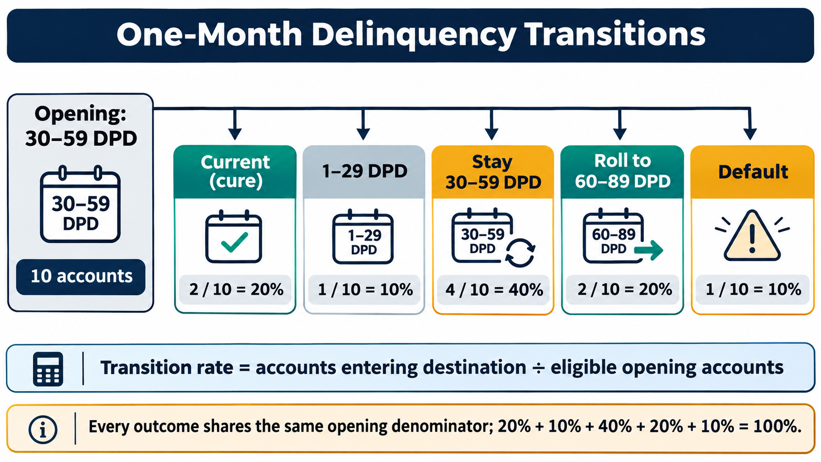
Start with the 10 accounts in 30–59 DPD. At the next monthly snapshot, each account has one of five outcomes. The shared denominator makes the row add to 100%.
🧭 AT A GLANCE · WHAT EACH RATE ANSWERS
Transition rate: Of accounts in opening state i, what fraction is in destination state j at the next observation?
Forward roll rate: What fraction moved from an opening delinquency bucket into a specified more severe bucket?
Cure rate: What fraction of accounts that started delinquent returned to the chosen current or healthier state?
Balance-weighted rate: What share of opening dollars, rather than accounts, moved to a destination?
1 · DEFINE THE STATES AND OBSERVATION WINDOW
A days-past-due (DPD) bucket classifies an account by how late its contractual payment is under a stated counting and payment-allocation rule. A transition matrix records the movement between these states. For example: Current, 1–29 DPD, 30–59 DPD, 60–89 DPD, policy-defined Default, and Closed/Other exit.
Choose mutually exclusive states that cover the outcomes you need to monitor. Decide whether “monthly” means calendar month-end, a fixed number of days, or the next statement date. Apply the same rule in both snapshots. An account may skip a bucket, cure, default directly, or exit; do not assume it moves only one step.
Keep delinquency buckets separate from the approved default definition. For Basel IRB, default includes an unlikeliness-to-pay assessment and a more-than-90-days-past-due criterion on a material credit obligation, subject to the applicable framework and supervisory rules. IFRS 9 separately has rebuttable presumptions concerning default no later than 90 days past due and significant increase in credit risk after more than 30 days past due. The latter is a backstop for staging assessment, not a universal default label. Delinquency is a lagging signal, so use earlier risk information where available.
Before counting, specify the unit (account, facility, borrower, or balance), opening-state rule, ending-state rule, default and exit treatment, cure definition, and handling of missing or immature records.
2 · BUILD THE TRANSITION MATRIX
Count eligible units by opening state and next-snapshot destination. Let n(i,j) be the count that starts in state i and ends in state j; let n(i) be all eligible units that start in i.
For each opening state, divide the count that reaches destination j by all eligible accounts that began in state i. This makes the denominator explicit and keeps each row comparable.
In the synthetic row below, 10 accounts begin in 30–59 DPD. Two reach 60–89 DPD, so that particular transition is 2 divided by 10. The opening count—not the ending total and not the full portfolio—is the denominator.
🔢 SYNTHETIC ONE-MONTH TRANSITION COUNTS
Current at opening (100 accounts): 90 Current; 7 at 1–29 DPD; 2 at 30–59 DPD; 0 at 60–89 DPD; 1 Default.
1–29 DPD at opening (20 accounts): 8 Current; 7 remain at 1–29 DPD; 4 at 30–59 DPD; 1 at 60–89 DPD; 0 Default.
30–59 DPD at opening (10 accounts): 2 Current; 1 at 1–29 DPD; 4 remain at 30–59 DPD; 2 at 60–89 DPD; 1 Default.
60–89 DPD at opening (5 accounts): 1 Current; 0 at 1–29 DPD; 0 at 30–59 DPD; 2 remain at 60–89 DPD; 2 Default.
Each row reconciles to its opening count. When the states are exhaustive and every unit has an observed destination, the transition percentages in each row sum to 100%. If closed, sold, transferred, or unobservable accounts are excluded, disclose that and show the denominator reconciliation; an unexplained missing share can bias the rates.
📈 3 · CALCULATE A FORWARD ROLL RATE
A forward roll rate must name both the starting bucket and destination. “30–59 to 60–89 DPD” is clear; “the roll rate” alone is ambiguous. Here, 2 of the 10 accounts starting in 30–59 DPD move to 60–89 DPD.
Worked result: 2 of the 10 opening accounts move from 30–59 DPD to 60–89 DPD, so the selected roll rate is 20%.
The same opening row also has one direct transition to Default, or 10%. Include skipped-bucket transitions when they matter; looking only at adjacent delinquency buckets would miss that direct movement.
For a complete destination rate, the same denominator is used for every outcome in the row:
Return to Current: 2 accounts, or 20% of the opening 10
Improve to 1–29 DPD: 1 account, or 10% of the opening 10
Remain in 30–59 DPD: 4 accounts, or 40% of the opening 10
Roll to 60–89 DPD: 2 accounts, or 20% of the opening 10
Enter Default: 1 account, or 10% of the opening 10
The five shares total 100%. “Remain” is a transition too: it measures persistence in the same state.
↩️ 4 · CALCULATE ONE-SNAPSHOT AND SUSTAINED CURE RATES
A cure rate needs an explicit cure definition. A one-snapshot cure is delinquent at the opening date and Current at the next observation. It does not prove the account stays current afterward.
For a selected opening delinquency state, divide the accounts that reach Current by the eligible accounts that began in that state.
Using the example counts: 8 of 20 accounts in 1–29 DPD return to Current (40%); 2 of 10 in 30–59 DPD return to Current (20%); and 1 of 5 in 60–89 DPD returns to Current (20%). Across these three opening delinquency buckets, 11 of 35 accounts return to Current, or 31.4%. Always show the bucket-level rates alongside a pooled figure, since the mix of starting buckets can change the pooled result.
A sustained cure could require the account to remain Current for, say, three consecutive monthly snapshots. That is a different outcome definition: follow accounts for the full three months, specify what happens if they default or close during follow-up, and do not count incomplete follow-up as a successful cure.
💰 5 · CHOOSE ACCOUNT OR BALANCE WEIGHTING
Account weighting answers “What share of accounts moved?” Balance weighting answers “What share of opening dollars moved?” Keep the unit explicit and do not mix the two.
Suppose the 10 accounts in the 30–59 DPD opening bucket have a total opening balance of $20,000. The two accounts that roll to 60–89 DPD have $6,000 of combined opening balance. The account roll rate is 20%; the balance roll rate is 30%. Both can be useful, but they describe different exposure concentrations.
For a balance-weighted transition, divide the opening balance that moves from i to j by the total eligible opening balance in i.
For the example, $6,000/$20,000 = 30%. Use the opening balance consistently in numerator and denominator, and state whether the balance is principal, gross carrying amount, or another defined exposure measure.
🔄 6 · EXTEND A ONE-MONTH MATRIX ACROSS MULTIPLE MONTHS
A transition matrix can be used to project future state distributions under explicit assumptions. With row-vector notation, let π₀ be the opening share across states and P the one-period transition matrix. Then:
Multiply the opening state distribution by the one-period matrix to estimate the next period. To project two periods with an unchanged matrix, apply the matrix a second time.
In the small example, start with 100 current accounts. Applying the Current row once gives an expected month-one mix of 90 Current, 7 at 1–29 DPD, 2 at 30–59 DPD, 0 at 60–89 DPD, and 1 Default. If the same transition rates are assumed to apply again, month two adds 0.9 expected defaults from the 90 Current accounts and 0.2 from the 2 accounts at 30–59 DPD. That is 1.1 expected new defaults. Including the first-month default, the two-month cumulative expected default share is 2.1% of the original 100 accounts.
This is a simple expected-count projection, not a prediction of fractional real accounts. It assumes the transition behavior is stationary over both months, default is absorbing, closed accounts are excluded, and the example probabilities adequately represent the same population. Real portfolios may need time-varying matrices, seasonality, changing macroeconomic conditions, competing exits, and confidence ranges. Matrix-projected default shares are not automatically a calibrated one-year PD.
📊 7 · MONITOR THE RATES RESPONSIBLY
Reconcile the population. Report opening counts and balances, missing records, closures, sales, and exclusions for every cohort.
Compare like with like. Fix state definitions, observation timing, product scope, unit, and denominator across reporting periods.
Review both transitions and persistence. Track forward rolls, cures, stays, direct defaults, and exits—not only the most severe transition.
Segment with care. Compare product, vintage, geography, channel, and approved risk segments only where samples are large enough. Show counts and uncertainty; small denominators make rates volatile.
Investigate changes before reacting. Check payment posting, DPD logic, holidays, servicing changes, policy actions, collections activity, and source-system coverage.
Separate operational monitoring from model validation. Roll rates can inform analysis of default dynamics, but a model PD needs its own target, horizon, calibration, validation, and governance.
A rising roll rate can reflect worsening borrower behavior, a changed denominator, a timing shift, or a data process change. Treat the statistic as a signal to investigate, not as a diagnosis by itself.
⚖️ 8 · KEEP THE MEASUREMENT PURPOSES DISTINCT
Collections and portfolio monitoring: Roll and cure rates summarize observed movement between operational states.
PD estimation: Transition data may support a model, but the resulting probability of default must have a defined default event, population, horizon, and calibration method.
IFRS 9 ECL: Expected credit loss measures probability-weighted contractual cash shortfalls using the applicable accounting requirements. A delinquency roll rate alone is not ECL; it may be one input among governed data and models.
Regulatory capital: Prudential rules define the relevant default, estimation, and use requirements. An internal operational matrix is not automatically an approved regulatory parameter.
📚 SOURCES AND SCOPE
Basel Framework, CRE36: IRB approach—minimum requirements. Default definition and prudential scope.
Basel Committee, guidance on credit risk and accounting for expected credit losses, PAP20. Paragraphs 20.82–20.83 discuss the IFRS 9 default presumption and default indicators; paragraphs 20.128–20.131 explain the more-than-30-days-past-due rebuttable presumption as a backstop and note that delinquency is a lagging indicator.
IFRS Foundation, IFRS 9 Financial Instruments. Standard overview and authoritative source for the applicable accounting requirements.
Educational methodology only. Definitions, thresholds, exclusions, and actions must follow the applicable portfolio policy, accounting framework, jurisdiction, and supervisory requirements.
📋 COPYABLE FORMULA REFERENCE
Try a reproducible Python example
These examples use synthetic inputs and run locally in a browser worker. Edit the code, run it, and compare its output with the published example.
Runnable Python · local in your browser
Compare expected loss and uncertainty across two distributions
Calculate the probability-weighted mean, variance, and standard deviation for two fully synthetic loss distributions.
Output
Run the code to see the output.
Runtime loads only after you press Run. Code runs in a separate browser worker with a 10-second limit and a 20,000-character output cap. Use synthetic examples only; browser execution is not a secure environment for secrets or sensitive records.
Runnable Python · local in your browser
Calculate WOE and IV from grouped counts
Use synthetic good and bad counts for three ordered scorecard bins. The 0.5 adjustment avoids a zero distribution in this small example.
Output
Run the code to see the output.
Runtime loads only after you press Run. Code runs in a separate browser worker with a 10-second limit and a 20,000-character output cap. Use synthetic examples only; browser execution is not a secure environment for secrets or sensitive records.
Educational material only. Methods and examples are simplified; state and validate the assumptions required for your use case.