Credit risk foundations
Credit Portfolio Stress Testing: A Step-by-Step Scenario Walkthrough
Work through a synthetic credit portfolio stress test: build a coherent adverse scenario, calculate segment losses, explain the drivers, and monitor key assumptions. Distinguishes internal stress sensitivities from IFRS 9 ECL and regulatory capital.
Updated 2026-11-11
Purpose
Work through a synthetic credit portfolio stress test: build a coherent adverse scenario, calculate segment losses, explain the drivers, and monitor key assumptions. Distinguishes internal stress sensitivities from IFRS 9 ECL and regulatory capital.
Key terms
Hover over or focus a term for a quick definition, or open its glossary entry.
EL = Σᵢ (EADᵢ × PDᵢ × LGDᵢ)
Baseline arithmetic: $220,000 × 2.5% × 40% = $2,200.
Stress arithmetic: $220,000 × 6.0% × 55% = $7,260.
Change in loss = stressed total − baseline total = $19,890 − $6,250 = $13,640.
Stress multiple = $19,890 ÷ $6,250 = 3.18 times baseline.
Percentage increase = $13,640 ÷ $6,250 = 218.24%.
Segment contribution = (stressed segment loss − baseline segment loss) ÷ total increase in loss.
◆ AT A GLANCE
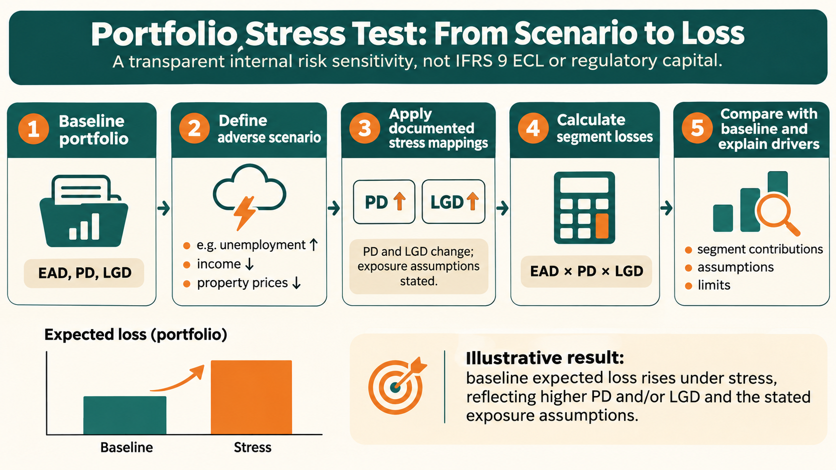
Stress testing asks how credit losses or other risk measures could change under a defined adverse scenario. This guide works a small synthetic portfolio through a one-period exposure at default (EAD) × probability of default (PD) × loss given default (LGD) sensitivity. The scenario has no assigned probability, so its result is conditional—not a probability-weighted forecast.
All figures below are synthetic and illustrative. This is an internal sensitivity, not an IFRS 9 expected credit loss (ECL) amount or a regulatory capital result.
◆ 1. DEFINE THE DECISION AND MEASURE
State what the exercise should inform: product vulnerabilities, risk appetite, collections capacity, portfolio limits, or management discussion. Fix the as-of date, portfolio scope, exposure unit, horizon, and output before selecting shocks.
Simple one-period loss proxy
This multiplies each segment's exposure by its default probability over the stated period and loss fraction if default occurs. It is a simplified representation under those assumptions, not a full valuation of contractual cash shortfalls.
◆ 2. WRITE A COHERENT ADVERSE SCENARIO
For illustration, assume rising unemployment, lower borrower income, and falling property prices. These shocks are invented for this example, not an economic forecast.
• Describe the event and its relevance to this portfolio.
• Choose the period and portfolio snapshot affected.
• Map the narrative to documented input changes. Here, PD and LGD rise by segment while EAD stays fixed.
• Challenge whether exposure should also change: revolving borrowers may draw more, customers may repay, and limits or collateral may move.
• Record data sources, model version, mapping method, exclusions, and adjustments.
Make the scenario severe enough to reveal vulnerabilities and internally consistent with its narrative. Basel Committee guidance highlights relevant risk coverage, coherent scenarios, clear assumptions and limitations, and periodic review.
◆ 3. CALCULATE THE SEGMENT RESULTS
Use a one-year horizon and fixed EAD. No scenario probability is assigned. Every amount and rate below is synthetic.
• Prime mortgage: EAD $150,000; baseline PD 1.5%, LGD 20%, loss $450; stress PD 3%, LGD 30%, loss $1,350; increase $900.
• Unsecured cards: EAD $60,000; baseline PD 4%, LGD 75%, loss $1,800; stress PD 8%, LGD 85%, loss $4,080; increase $2,280.
• Small business: EAD $220,000; baseline PD 2.5%, LGD 40%, loss $2,200; stress PD 6%, LGD 55%, loss $7,260; increase $5,060.
• Commercial property: EAD $400,000; baseline PD 1.8%, LGD 25%, loss $1,800; stress PD 4.5%, LGD 40%, loss $7,200; increase $5,400.
Total EAD is $830,000. Baseline loss is $6,250; stressed loss is $19,890; the increase is $13,640.
Example: small-business baseline
Example: small-business stress
Portfolio change
The 3.18× ratio describes this synthetic arithmetic; it does not predict realized loss.
◆ 4. EXPLAIN WHAT DRIVES THE CHANGE
Commercial property contributes $5,400 of the $13,640 increase, and small business contributes $5,060. Together that is 76.7% of the modeled increase. Check whether these exposures cluster in vulnerable industries or regions, whether collateral values could fall together, and whether undrawn facilities could increase exposure.
Share of total increase from segment i
This is a share of the modeled change, not proof of causation. Where inputs interact nonlinearly, rerun controlled counterfactuals before attributing the result to one factor. For practice, hold LGD at baseline and change only PD; then restore PD and change only LGD. Compare those sensitivities with the combined scenario.
◆ 5. BUILD THE WORKFLOW
• Set scope: portfolio, as-of date, unit, horizon, and decision use.
• Write the scenario: explain the event and portfolio vulnerabilities.
• Check consistency: align assumptions for employment, income, arrears, collateral, and utilization.
• Map risk drivers: document method, source, segment, horizon, and limitations for each changed input.
• Calculate and reconcile: reproduce baseline, calculate stress outputs, and reconcile both totals to source data.
• Challenge and report: show drivers, uncertainty, exclusions, model limits, and plausible management responses.
• Review: refresh scenarios when portfolio composition, vulnerabilities, or economic conditions change.
◆ 6. MONITOR COVERAGE, ASSUMPTIONS, AND OUTPUTS
• Portfolio coverage: included EAD share and excluded exposure. Ask whether material products, regions, and commitments are represented.
• Scenario integrity: shock values, units, horizon, and dependency checks. Ask whether related assumptions are coherent.
• Input sensitivity: loss change as PD, LGD, or EAD shocks vary. Identify the assumptions that dominate the result.
• Concentration: each segment's share of stressed loss and incremental loss. Check if a small portfolio slice drives most of the impact.
• Data and model quality: reconciliation breaks, missing or stale inputs, and model version. Confirm the result can be reproduced.
• Decision use: action, accountable owner, due date, and follow-up. Record whether analysis informed a decision and was acted on.
Set escalation limits for the institution's purpose and governance. No single PSI value, loss multiple, or percentage threshold universally proves a scenario or model acceptable. Review narrative, coverage, assumptions, model uncertainty, and decisions together.
◆ 7. KEEP THE MEASURES DISTINCT
• Internal stress sensitivity: a conditional loss proxy under one scenario, with no scenario probability applied.
• IFRS 9 ECL: accounting measurement has its own requirements, including probability-weighted forward-looking measurement. One severe scenario without appropriate weighting and measurement design is not an ECL allowance.
• Regulatory capital: prudential capital and supervisory stress tests use their own definitions, portfolios, assumptions, and rules. This simple calculation does not produce a capital requirement.
Do not label the $19,890 scenario result an allowance, forecast, or capital requirement. Keep scope, assumptions, model version, and limitations with every result.
◆ LIMITATIONS
This single-horizon approximation holds exposure fixed and has four synthetic segments. It omits default correlation, portfolio migration, loss timing and discounting, changing exposures, commitments, recovery timing, model uncertainty, feedback, and management actions. Severe stress can be nonlinear, and past relationships may weaken in future conditions.
◆ REFERENCES
• Basel Committee on Banking Supervision, Basel Consolidated Guidelines: Stress testing — risk-management use, coherent scenarios, risk coverage, assumptions, limitations, and periodic review.
• Basel Committee on Banking Supervision, Basel Consolidated Guidelines: General credit risk management — Principle 12 addresses forward-looking market and macroeconomic factors and stressed credit exposures.
Educational material only. All scenario inputs are synthetic. Adapt scope, assumptions, and controls to the intended use and applicable requirements.
Try a reproducible Python example
These examples use synthetic inputs and run locally in a browser worker. Edit the code, run it, and compare its output with the published example.
Runnable Python · local in your browser
Compare expected loss and uncertainty across two distributions
Calculate the probability-weighted mean, variance, and standard deviation for two fully synthetic loss distributions.
Output
Run the code to see the output.
Runtime loads only after you press Run. Code runs in a separate browser worker with a 10-second limit and a 20,000-character output cap. Use synthetic examples only; browser execution is not a secure environment for secrets or sensitive records.
Runnable Python · local in your browser
Calculate WOE and IV from grouped counts
Use synthetic good and bad counts for three ordered scorecard bins. The 0.5 adjustment avoids a zero distribution in this small example.
Output
Run the code to see the output.
Runtime loads only after you press Run. Code runs in a separate browser worker with a 10-second limit and a 20,000-character output cap. Use synthetic examples only; browser execution is not a secure environment for secrets or sensitive records.
Educational material only. Methods and examples are simplified; state and validate the assumptions required for your use case.