Credit risk foundations
Measuring Credit Portfolio Concentration: HHI, Exposure Shares, and Stress Tests
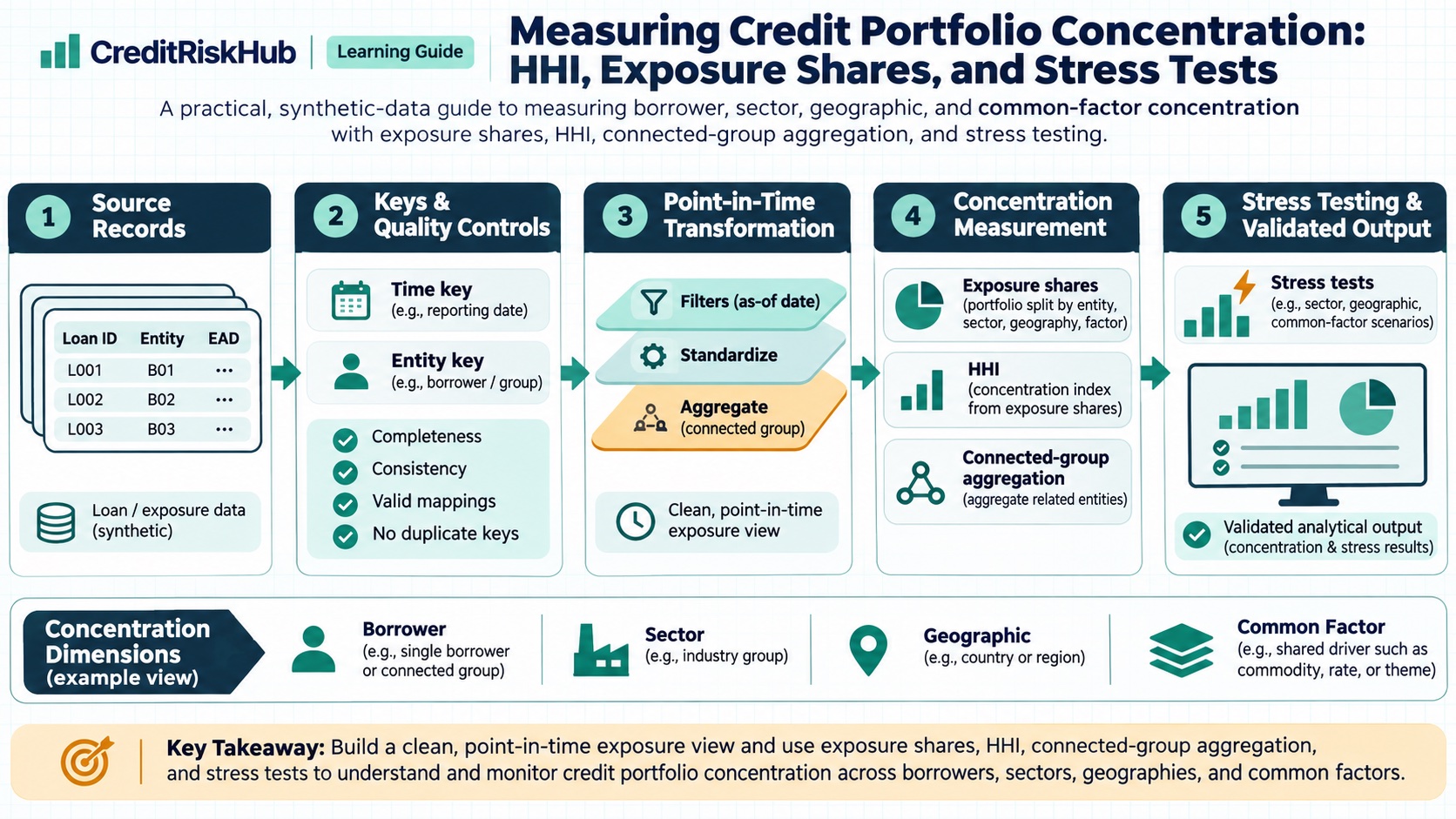
A practical, synthetic-data guide to measuring borrower, sector, geographic, and common-factor concentration with exposure shares, HHI, connected-group aggregation, and stress testing.
Updated 2026-10-25
Purpose
A practical, synthetic-data guide to measuring borrower, sector, geographic, and common-factor concentration with exposure shares, HHI, connected-group aggregation, and stress testing.
Key terms
Hover over or focus a term for a quick definition, or open its glossary entry.
Suppose four independent-looking borrower records have exposures of 400, 300, 200, and 100 units. Total exposure is 1,000. Shares are 40%, 30%, 20%, and 10%. Name HHI = 0.40² + 0.30² + 0.20² + 0.10² = 0.30, or 3,000 on the 0–10,000 scale. The largest name is 40%; the top two are 70%; effective number = 1 / 0.30 = 3.33.
A sector HHI is calculated from sector shares, not the borrower shares. If those same exposures fall into sectors with 700 and 300 units, sector HHI is 0.70² + 0.30² = 0.58 (5,800). Each HHI answers a different grouping question. Do not compare values without matching the population, exposure basis, and grouping definitions.
Synthetic one-year sensitivity: assume sector X has EAD 700, PD 2%, and LGD 45%; sector Y has EAD 300, PD 1%, and LGD 30%. Baseline simple expected loss is 700 × 2% × 45% + 300 × 1% × 30% = 7.2 units. If a stress raises only sector X PD to 8%, keeping EAD and LGD fixed, the stressed total is 700 × 8% × 45% + 300 × 1% × 30% = 26.1 units; the incremental sensitivity is 18.9 units.
PURPOSE
Credit concentration risk is the risk that exposures share a borrower, connected group, sector, geography, product, collateral source, or other common driver, so adverse conditions can create losses larger than a diversified portfolio view suggests. A portfolio can have many loans and still depend heavily on a small number of related risks.
This guide builds a practical concentration dashboard from exposure shares, top-N shares, and the Herfindahl–Hirschman Index (HHI), then adds a transparent stress sensitivity. All data below are synthetic. Basel guidance describes concentration categories and calls for documented definitions, limits, and periodic stress tests for banks within its supervisory scope. This educational workflow is not a regulatory limit calculation or a substitute for applicable local requirements.
STEP 1 — DEFINE THE PORTFOLIO AND EXPOSURE BASIS
Freeze the reporting date, entity perimeter, products, currency conversion date, inclusion rules, and grain (facility, borrower, or group). Choose a consistent exposure measure, such as drawn balance plus a defined credit-conversion treatment for undrawn commitments. Record how guarantees, collateral, accrued interest, securitizations, and off-balance-sheet items are represented. Do not mix gross exposure in one segment with net exposure in another without showing both.
Reconcile totals to the source ledger or risk system. Keep the original facility and obligor identifiers, reporting timestamp, currency, and transformation version so another analyst can reproduce the result. Missing or unresolved obligor links should be visible as an “unknown” bucket rather than silently excluded.
STEP 2 — AGGREGATE CONNECTED COUNTERPARTIES
A legal-entity count can understate concentration when several entities depend on the same parent, cash flow, or economic relationship. Build a governed mapping from facility to legal obligor and from obligor to connected group. Preserve the mapping’s effective dates, evidence, owner, and confidence. Review new entities, mergers, ownership changes, and exceptions. If group membership is uncertain, show an alternative aggregation or sensitivity.
Avoid counting the same exposure twice within one metric. An exposure may appear in several separate views—for example, both its connected group and its sector—but those are different lenses and must not be added together as if they were disjoint portfolio slices.
STEP 3 — BUILD COMPLEMENTARY EXPOSURE METRICS
For exposure Eᵢ and total exposure E, the share for name i is sᵢ = Eᵢ / E. Top-N share is the sum of the N largest exposure amounts divided by E. These are easy to explain and useful for tracking large names, but they say nothing by themselves about default likelihood, recovery, or correlation.
The name HHI is HHI = Σ sᵢ². It ranges from close to zero for many similarly sized names up to 1 for a single name. Multiply by 10,000 for the commonly used 0–10,000 presentation scale. The reciprocal, 1 / HHI, is an “effective number of equally sized names” that can make a portfolio comparison intuitive. It is a descriptive summary, not a count of actual borrowers, a safe concentration threshold, or a regulatory capital measure.
Calculate separate views by connected group, sector, geography, product, currency, collateral type, guarantor, and any material common activity or commodity. Basel identifies single counterparties and connected groups, common industries or regions, shared activities or commodities, and concentrations in collateral or credit protection as relevant lenses. Use the categories that make sense for the portfolio and document them.
STEP 4 — WORKED SYNTHETIC HHI EXAMPLE
If the first two borrowers are actually one connected group, group exposures are 700, 200, and 100. Group HHI becomes 0.70² + 0.20² + 0.10² = 0.54, or 5,400. The legal-obligor view did not change; the connected-group view reveals the dependency that the first calculation missed.
STEP 5 — COPYABLE PYTHON CALCULATION
This deterministic Python 3 example uses four fixed synthetic exposures and only the standard library. It has no network, file, or system access.
exposures = {"Borrower A": 400.0, "Borrower B": 300.0, "Borrower C": 200.0, "Borrower D": 100.0}
total = sum(exposures.values())
shares = {name: amount / total for name, amount in exposures.items()}
hhi = sum(share ** 2 for share in shares.values())
top_two_share = sum(sorted(exposures.values(), reverse=True)[:2]) / total
effective_names = 1 / hhi if hhi else 0
print("Total exposure:", total)
print("Largest-name share:", max(shares.values()))
print("Top-two share:", top_two_share)
print("HHI (0–1):", hhi)
print("HHI (0–10,000):", hhi * 10000)
print("Effective number of names:", effective_names)
Expected results: total 1,000; largest-name share 0.4; top-two share 0.7; HHI 0.3; scaled HHI 3,000; effective number about 3.33. To calculate a group or sector view, first aggregate the exposure dictionary by the governed group or sector key, then apply the same share formula. Do not use this small example as a production limit engine.
STEP 6 — ADD RISK SENSITIVITY WITHOUT MISLABELING IT
Exposure HHI treats every unit equally. Add complementary internal views where data and purpose support them: expected-loss contributions EAD × PD × LGD, stressed losses by segment, rating or vintage mix, and exposure-weighted concentration under adverse scenarios. Name the measure and assumptions explicitly; a PD/LGD-weighted sensitivity is not the same as an exposure HHI.
This is an illustrative one-period expected-loss sensitivity, not IFRS 9 ECL, Basel regulatory expected loss, or regulatory capital. It omits scenario probability weighting, discounting, changing exposures and recoveries, default dependence, management actions, and other effects. Accounting ECL requires the applicable accounting framework and reporting-date assumptions; prudential capital follows applicable regulatory rules; an internal concentration stress supports a separate risk-management decision. Do not interchange these outputs because they use similar PD, LGD, or EAD inputs.
STEP 7 — TURN THE NUMBERS INTO MONITORING
A useful monthly or quarterly pack can track: total exposure and reconciliation difference; largest-name and top-N shares; name and connected-group HHI; sector and geography shares; limit utilization and days in breach; unknown or unmapped exposure; new or changed connected-group links; exposures near limits; baseline and stressed loss by material segment; and movement from the prior reporting date. Show both amount and percentage, denominators, date, segment count, and change from a fixed comparison period.
Set thresholds through approved risk appetite and portfolio materiality; no single HHI or top-name value is universally safe. Escalation triggers should lead to investigation: validate the data and grouping, identify the drivers, compare baseline and stress results, assess portfolio capacity and customer impact, then document the accountable owner, decision, and review date. Do not automatically reject or sell a sound exposure solely to improve a summary statistic.
STEP 8 — DESIGN A MEANINGFUL STRESS TEST
Start from a plausible vulnerability, such as a regional employment shock, commodity-price fall, major employer failure, property-market decline, or collateral-provider impairment. State the scenario horizon, affected segments, PD/LGD/EAD changes, correlation or common-factor assumption, and any management actions. Calculate stressed loss and compare it with a clearly named internal capacity measure. Run sensitivities where the scenario or group mapping is uncertain. Basel supervisory guidance expects banks to document how relevant concentrations and limits are defined and calculated and to periodically stress-test major concentrations; the exact regulatory application depends on jurisdiction and institution.
STEP 9 — DATA AND GOVERNANCE CHECKS
Before publishing a metric, test that exposures sum to the source, IDs are stable, connected-group mapping is current, sector codes are populated, currency conversion is consistent, undrawn amounts follow the chosen rule, and every reporting date uses the same scope. Version the mapping, metric definitions, thresholds, source extract, code, and approvals. Explain breaks in trend caused by acquisitions, taxonomy changes, portfolio transfers, or restatements rather than presenting them as economic movement.
LIMITATIONS AND INTERPRETATION
HHI is sensitive to grouping and data completeness. It does not encode correlation between apparently different names, probability of default, loss severity, tenor, collateral dependence, or the severity of a common shock. A diversified portfolio can still be exposed to one macro factor; a concentrated one may be adequately compensated or supported by mitigants. Read concentration measures with credit quality, scenario analysis, limits, and portfolio context. Small or changing portfolios can produce noisy ratios.
REFERENCES
Basel Committee on Banking Supervision, General credit risk management (Basel Consolidated Guidelines), especially the concentration-risk discussion and stress-testing guidance: https://www.bis.org/committees/bcbs/basel-consolidated-guidelines/module/cri/10
Basel Framework, SRP 32 — Credit risk, paragraphs 32.8–32.13 (concentration definitions, documented frameworks, limits, stress tests, and Pillar 2 assessment): https://www.bis.org/committees/bcbs/basel-framework/standard/srp/32/inforce/2023-01-01/published/2020-03-27
Educational material only. Synthetic amounts and assumptions do not represent a real borrower or portfolio. Confirm local supervisory rules, accounting requirements, exposure definitions, and risk appetite before operational use.
Try a reproducible Python example
These examples use synthetic inputs and run locally in a browser worker. Edit the code, run it, and compare its output with the published example.
Runnable Python · local in your browser
Compare expected loss and uncertainty across two distributions
Calculate the probability-weighted mean, variance, and standard deviation for two fully synthetic loss distributions.
Output
Run the code to see the output.
Runtime loads only after you press Run. Code runs in a separate browser worker with a 10-second limit and a 20,000-character output cap. Use synthetic examples only; browser execution is not a secure environment for secrets or sensitive records.
Runnable Python · local in your browser
Calculate WOE and IV from grouped counts
Use synthetic good and bad counts for three ordered scorecard bins. The 0.5 adjustment avoids a zero distribution in this small example.
Output
Run the code to see the output.
Runtime loads only after you press Run. Code runs in a separate browser worker with a 10-second limit and a 20,000-character output cap. Use synthetic examples only; browser execution is not a secure environment for secrets or sensitive records.
References
- Basel Committee on Banking Supervision — Basel Committee on Banking Supervision
Educational material only. Methods and examples are simplified; state and validate the assumptions required for your use case.