Credit-risk data engineering
Feature Engineering for Credit Risk: Behavioral Windows Without Leakage
Build point-in-time-safe credit-risk features from payment behavior, balances, delinquencies, categories, trends, and missing data. Includes a worked synthetic example, browser-safe Python, leakage controls, and a production monitoring checklist.
Updated 2026-11-11
Purpose
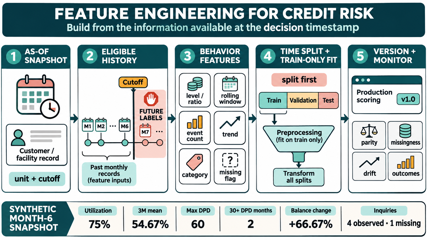
Build point-in-time-safe credit-risk features from payment behavior, balances, delinquencies, categories, trends, and missing data. Includes a worked synthetic example, browser-safe Python, leakage controls, and a production monitoring checklist.
Key terms
Hover over or focus a term for a quick definition, or open its glossary entry.
Utilizationutilizationₜ = balanceₜ ÷ limitₜ
Relative balance trendtrend₃ₘ = (balanceₜ − balanceₜ₋₃) ÷ balanceₜ₋₃
Detailed explanation
At a glance
Only use point-in-time data: every feature must reflect what was known at the prediction date. Examples below use synthetic records.
Related terms: data quality, days past due (DPD), and probability of default (PD).
1. Define the prediction moment first
Choose the observation unit: application, obligor, or facility. Align its grain with the modeled outcome.
Set an as-of timestamp and include only records both effective and available by that point. A late-arriving record must not leak into an earlier snapshot.
Define the outcome window separately, such as default in the 12 months after the snapshot. Exclude future outcome fields from the feature table.
Specify window completeness. For a six-month summary, require six valid months or explicitly document a partial-window rule.
Version the source fields, cutoffs, null rules, units, transformations, and feature definitions.
Eligible historyevent_time ≤ as_of_time AND available_time ≤ as_of_time
An event date alone may not prove that information was available to a decision system. Use an ingestion or availability timestamp when a source can arrive late or be corrected retrospectively.
2. Common feature families and design checks
FamilySynthetic exampleCalculation ideaDesign check
Level or ratio
Current utilization
Balance ÷ current limit
Define zero, missing, stale, and changed limits.
Window summary
Mean utilization over 3 months
Mean of month-end ratios
Track the number of valid periods.
Event count
Months at 30+ DPD in 6 months
Count months meeting the condition
A month count is not an episode count.
Recency
Months since latest 30+ DPD
As-of month minus last event month
Represent “no prior event” separately.
Trend
Balance change over 3 months
Change ÷ earlier balance
Define zero-base and irregular-time behavior.
Categorical
Product type
Stable one-hot flags or mapping
Preserve unknown and unseen categories.
Missingness
Inquiry count unavailable
Observed-value flag
Distinguish missing from a true zero.
Interaction
High utilization with recent delinquency
Combine documented features
Check rationale, stability, and interpretability.
Every ratio needs a numerator, denominator, unit, and zero-denominator rule. Fit imputation, scaling, capping, bins, feature selection, and category mappings on training data only, then apply the saved transformations to later data.
3. Worked example: a month-6 account snapshot
All rows are synthetic. The target outcome is not used to calculate these features.
MonthBalanceLimitDPDInquiries
1
$4,000
$10,000
0
1
2
$4,200
$10,000
0
0
3
$4,500
$10,000
30
Missing
4
$4,600
$10,000
60
2
5
$4,300
$10,000
0
1
6
$7,500
$10,000
0
0
FeatureCalculationResultInterpretation
Current utilization
$7,500 ÷ $10,000
75.00%
Month-6 balance divided by limit.
Mean utilization, months 4–6
(46% + 43% + 75%) ÷ 3
54.67%
Three month-end ratios.
Maximum DPD, months 4–6
max(60, 0, 0)
60
Month 4 had the highest days-past-due value in the window.
Months at 30+ DPD, months 1–6
Count months 3 and 4
2 months
A month count, not two delinquency episodes.
Balance change, months 3–6
($7,500 − $4,500) ÷ $4,500
+66.67%
Three-month relative change from month 3.
Observed inquiry total
1 + 0 + 2 + 1 + 0
4
Five reported values; month 3 is missing.
This is one account snapshot, not six independent model rows. A production dataset may contain multiple snapshots per account; handle overlapping outcome windows and repeated-account dependence.
4. Runnable Python: create the feature row
This deterministic example uses six synthetic records and Python built-ins only. It has no file, network, shell, or system access. The loop bounds are fixed by the six-row example.
history = [ {"month": 1, "balance": 4000, "limit": 10000, "dpd": 0, "inquiries": 1}, {"month": 2, "balance": 4200, "limit": 10000, "dpd": 0, "inquiries": 0}, {"month": 3, "balance": 4500, "limit": 10000, "dpd": 30, "inquiries": None}, {"month": 4, "balance": 4600, "limit": 10000, "dpd": 60, "inquiries": 2}, {"month": 5, "balance": 4300, "limit": 10000, "dpd": 0, "inquiries": 1}, {"month": 6, "balance": 7500, "limit": 10000, "dpd": 0, "inquiries": 0},]as_of_month = 6eligible = [r for r in history if r["month"] <= as_of_month]eligible.sort(key=lambda r: r["month"])assert len(eligible) == 6 and eligible[-1]["month"] == as_of_monthdef utilization(row): limit = row["limit"] return row["balance"] / limit if limit and limit > 0 else Nonecurrent = eligible[-1]last_three = eligible[-3:]recent_util = [utilization(r) for r in last_three]recent_util = [v for v in recent_util if v is not None]recent_dpd = [r["dpd"] for r in last_three]base = eligible[-4]["balance"]balance_change = (current["balance"] - base) / base if base else Noneinquiries = [r["inquiries"] for r in eligible]observed = [v for v in inquiries if v is not None]features = { "utilization_current": utilization(current), "utilization_mean_3m": sum(recent_util) / len(recent_util) if recent_util else None, "max_dpd_3m": max(recent_dpd) if recent_dpd else None, "months_30dpd_6m": sum(r["dpd"] >= 30 for r in eligible), "balance_change_3m": balance_change, "inquiries_6m_observed_sum": sum(observed), "inquiries_6m_missing": int(len(observed) != len(eligible)),}assert round(features["utilization_current"], 4) == 0.75assert round(features["utilization_mean_3m"], 4) == 0.5467assert features["max_dpd_3m"] == 60assert features["months_30dpd_6m"] == 2assert round(features["balance_change_3m"], 4) == 0.6667assert features["inquiries_6m_observed_sum"] == 4assert features["inquiries_6m_missing"] == 1for name, value in features.items(): print(f"{name}: {value}")
Expected key outputs: current utilization 0.75, three-month average 0.5467, maximum recent DPD 60, two 30+ DPD months in six months, balance trend 0.6667, inquiry sum 4, and missingness flag 1. In a production pipeline, also validate unique periods, ordering, late records, changed limits, currency units, empty histories, and parity between offline and serving calculations.
5. Prevent target leakage and train–serve mismatch
Split observations by time before fitting imputers, scalers, encoders, bins, or target-informed feature selection.
Build each row from a historical as-of snapshot. Exclude later default, collection, write-off, and bureau-update fields.
Start outcome windows after the as-of date. Exclude or correctly censor snapshots without a fully observed performance period.
Validate on later periods and, when appropriate, separate customers or facilities. Random row splits can put nearly identical snapshots on both sides.
Package preprocessing with the model and reuse the saved version at scoring time. Never refit it independently on validation, test, or production data.
Test boundaries: zero limits, missing fields, unseen categories, duplicate months, late arrivals, empty history, and dates around default.
Scikit-learn’s guidance recommends splitting before learned preprocessing, fitting transformations on training data, and applying the saved pipeline later. Pandas windowing supports rolling, time-based, and grouped calculations; match the endpoint and periods to the business definition.
6. Monitor the feature system after launch
ControlMeasureInvestigate when
Availability
Null rate, source coverage, stale-record share
Feeds change, missingness spikes, or values arrive after cutoff.
Validity
Range/domain violations; denominator failures
Values become impossible, limits are zero, or units change.
Distribution
Quantiles, category shares, PSI/CSI with documented bins
A change matters to the portfolio or model use. No universal threshold replaces review.
Window integrity
Valid periods, late records, duplicate observations
History length changes or periods repeat.
Transformation parity
Offline and production values on identical records
Mapping, version, timing, or rounding differs.
Predictive impact
Calibration and discrimination by vintage and segment
Drift aligns with changed outcomes or performance.
Governance
Inventory, owner, rationale, lineage, version, approval
A source, definition, or use changes without review.
Monitor raw inputs and derived features. A stable raw distribution can hide broken windowing, stale limits, or a changed missing-data rule. Pair drift signals with matured outcomes and a documented review action.
7. Keep the risk measure distinct
These features may support an internal application or behavioral PD model, monitoring, or another documented decision. A feature is not itself a PD estimate, an IFRS 9 expected credit loss, or a regulatory-capital measure. Accounting and prudential applications have distinct objectives and rules; data availability alone does not justify reusing one model.
Common mistakes
Including records posted after the decision cutoff.
Using a future default or collection field as a predictor.
Treating missing values as zero without justification.
Dividing by a zero, stale, or post-cutoff limit.
Fitting bins or imputers before the time split.
Treating overlapping account snapshots as independent.
Watching only AUC while ignoring data availability or calculation parity.
References
scikit-learn: Common pitfalls and recommended practices
pandas: Windowing operations
pandas: GroupBy and split-apply-combine
Educational material only. All records are synthetic. Set feature definitions, exclusions, validation design, and governance controls for the intended use.
Try a reproducible Python example
These examples use synthetic inputs and run locally in a browser worker. Edit the code, run it, and compare its output with the published example.
Runnable Python · local in your browser
Detect a point-in-time feature leak
A miniature data preparation check compares each feature's observation date with the prediction date.
Output
Run the code to see the output.
Runtime loads only after you press Run. Code runs in a separate browser worker with a 10-second limit and a 20,000-character output cap. Use synthetic examples only; browser execution is not a secure environment for secrets or sensitive records.
Runnable Python · local in your browser
Engineer numeric credit-risk features
Use a training-only median, explicit missingness flags, a log transform, a payment-to-income ratio, and a delinquency indicator. Amounts are synthetic CAD; transforms are illustrative and should be validated for the intended population.
Output
Run the code to see the output.
Runtime loads only after you press Run. Code runs in a separate browser worker with a 10-second limit and a 20,000-character output cap. Use synthetic examples only; browser execution is not a secure environment for secrets or sensitive records.
Educational material only. Methods and examples are simplified; state and validate the assumptions required for your use case.